Reference-based Multiple Imputation (2) - J2R and CR Methods
Missing data pattern
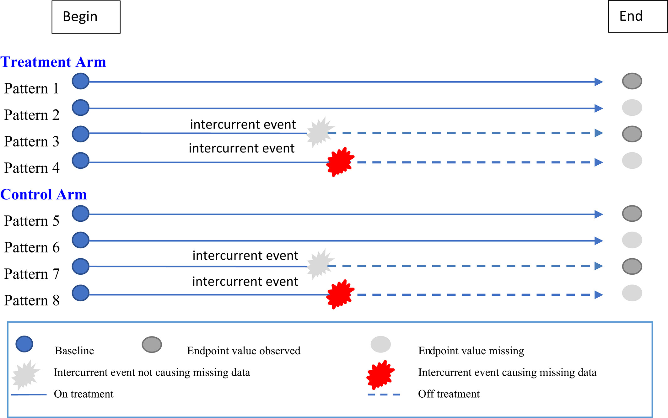
Basic notations
Let \(Y = [y_1, y_2, y_3, \dots, y_{J-1}, y_J]\) be an \(n\) by \(J\) matrix, where each column vector \(y_j = [y_{j,1}, y_{j,2}, \dots, y_{j,i}, \dots, y_{j,n-1}, y_{j,n}]^T\) records a continuous endpoint of interest (e.g., HbA1c in a diabetes trial) measured from \(n\) subjects at a pre-specified timepoint \(j\), for \(j = 1, \dots, J-1, J\). Specifically, \(y_1\) and \(y_J\) are the measurements taken at baseline and the primary timepoint of interest (e.g., HbA1c at Week 26), respectively.
In practice, \(y_1\) can be completely observed, but missing records in \(y_J\) are unavoidable.
Consider \(y_J = (y_J^{(obs)}, y_J^{(mis)})\), a partition of \(y_J\) into two parts consisting of the observed data \(y_J^{(obs)}\) and the missing data \(y_J^{(mis)}\).
Use \(X\) to denote covariates.
Jump to reference (J2R) method and Copy reference (CR) method
In placebo-controlled studies, two alternatives to the washout method (see previous post) are the jump-to-reference (J2R) and the copy reference (CR; see section below) approaches.
For these two methods, missing data from the control arm (Pattern 8) are imputed under the MAR assumption in the same fashion as the washout method that is,
\[ y_J \sim y_1^{obs}+y_{\text{int}}^{(obs)}+X \quad \text{(for the placebo arm).} \] The difference between the Washout, J2R, and CR methods is how intermediate measurements are used to impute missing data in the experimental arm (Pattern 4).
| Method | Uses Intermediate Data? | Core Assumption About Dropouts (Experimental Arm) | When Dropout Behavior Matches Control Arm |
| Washout | No (Discarded) | Relies strictly on available baseline and endpoint data to impute missing values. | N/A |
| Copy Reference (CR) | Yes | Subject loses experimental benefit and expects similar outcomes to the control group. | From the beginning of the study. (Note: 假设无论受试者实际上是何时退出的,实验组的脱落者从研究一开始其表现就与对照组相同。有一种“全盘否定”的感觉,假设这个患者只要退出了,就当他从第一天起就没吃过试验药,直接把对照组的数据特征复制(Copy)到他整个研究周期上。它忽略了患者退出前可能已经获得的药物疗效。) |
| Jump-to-Reference (J2R) | Yes | Subject loses experimental benefit and expects similar outcomes to the control group. | Only after the point of discontinuation. (Note: 假设实验组的脱落者只有在停止接受指定的治疗(EOT)之后,其表现才会与对照组相似。假设里“承认”患者在退出前是吃了试验药的(保留前期疗效)。但是一旦他们停药Dropout,他们的数据轨迹就会Jump到对照组的趋势上,表现得和对照组一样。) |
In the settings of placebo-controlled anti-hyperglycemic trials
In general, the J2R approach yields more conservative results than the CR approach if the experimental treatment has better treatment effect than the control treatment.
While extensive research exists on Jump to Reference (J2R) and Copy Reference (CR) methods, FDA statistical reviewers generally favor the Washout method for primary efficacy analyses in placebo-controlled antihyperglycemic trials.
Why the Washout method is preferred over the alternatives:
Washout Method (Preferred) – Computational Efficiency: It produces results similar to J2R but is computationally less intensive.
Conservativeness: It is generally more conservative than J2R. By completely “washing out” the effect of the experimental treatment, it avoids retaining partial treatment effects observed at intermediate timepoints (e.g., Week 12) before an intercurrent event.
Jump to Reference (J2R) – The Drawback: J2R imputes missing data conditional on intermediate measurements. Consequently, it does not fully remove the influence of the experimental treatment received prior to dropout, making it less conservative than the Washout method in certain scenarios. (Note: J2R保留了部分治疗效应,相比washout method不够保守)
Copy Reference (CR) – Unrealistic Assumption: CR assumes subjects in the experimental arm had the same mean response as the placebo group even before dropping out, which typically contradicts actual observations. Additionally, the analysis result based on the CR approach is not always conservative, which may increase the risk of an inflated type I error rate (Note: 这一点很反直觉).
Statistical methodology for J2R
Assume an unstructured multivariate normal (MVN) model with separate mean at each time point for each arm and a separate unstructured covariance matrix for each arm.
Assume monotone missingness and no missing data at baseline.
Based on the missing pattern, firstly divide subjects from the experimental arm with missing endpoint measurements into groups: \(G_1, ...,G_{J-1}\). Specifically, two subjects belong to the same group \(G_j\) if their last measurements before intercurrent events are taken at the same timepoint \(j \quad (j=1,2,...,J-1)\).
The J2R method assumes subjects in the experimental arm resemble subjects in the control arm immediately after the occurrence of intercurrent events.
For a subject \(g_j \in G_j\), the missing endpoint values \(y_{g_j, (j+1), \ldots, J}^{(\text{mis})} = \left( y_{\mathrm{g_j}, \mathrm{j}+1}^{(\text{mis})}, \ldots, y_{\mathrm{g_j}, \mathrm{J}}^{(\text{mis})} \right)^{\mathrm{T}}\) are imputed based on the following normal distribution (Note: 这里的意思是,同属于一个Group \(G_j\)的受试者,都会有相同的monotone missing pattern,因为上面已经假设了只有monotone missingness。这也暗示了,这类\(G_j\)里的受试者,他们在时间点\(j+1,...,J\)上,终点指标都是缺失的。因为ICE前最后一个测量在时间点\(j\),所以相应地,ICE后的第一个测量就在\(j+1\)。). See equation \(E1\) below:
\[ y_{g_j, (j+1)\ldots J}^{(\text{mis})} \sim N\left( \mu_{\text{PBO}, (j+1)\ldots J}^{(\text{obs})} + \Sigma_{21} \Sigma_{11}^{-1} \left( y_{g_j, 1\ldots j}^{(\text{obs})} - \mu_{G_j, 1\ldots j}^{(\text{obs})} \right), \Sigma_{22} - \Sigma_{21} \Sigma_{11}^{-1} \Sigma_{12} \right) \quad (\text{for the experimental arm, J2R}). \] Notations for the above distribution:
- The following is the mean vector of the observed values from the placebo completers at timepoints \(j+1,...,J\):
\[ \mu_{\text{PBO}, (j+1)\ldots J}^{(\text{obs})} = \left( \mu_{\text{PBO}, (j+1)}^{(\text{obs})}, \ldots, \mu_{\text{PBO}, J}^{(\text{obs})} \right)^T \]
- The following are the observed intermediate measurements at timepoints \(1,2,...,j\) for the subject \(g_j \in G_j\).
\[ y_{g_j, 1\ldots j}^{(\text{obs})} = \left( y_{g_j, 1}^{(\text{obs})}, \ldots, y_{g_j, j}^{(\text{obs})} \right)^T \] - The following is the mean vector at timepoints \(1,2,...,j\) for all subjects in group \(G_j\).
\[ \mu_{G_j, 1\ldots j}^{(\text{obs})} = \left( \mu_{G_j, 1}^{(\text{obs})}, \ldots, \mu_{G_j, j}^{(\text{obs})} \right)^T \]
- For the matrix stuff…..
Let \(\Sigma = \begin{bmatrix} \Sigma_{11} & \Sigma_{12} \\ \Sigma_{21} & \Sigma_{22} \end{bmatrix}\) be the \(J\times J\) sample covariance matrix based on data from placebo completers at timepoints \(1,2,...,J\).
The \(\Sigma\) is partitioned based on \(j\), the timepoint at which the last measurement before the ICEs is taken.
Specifically:
The matrix \(\Sigma_{11} = \text{cov} \left( y_{{\text{PBO}}, 1\ldots j}^{(\text{obs})} \right)\) is the \(j \times j\) sample covariance matrix based on placebo completers at timepoints \(1,2,...,j\).
The matrix \(\Sigma_{22} = \text{cov} \left( y_{\text{PBO}, (j+1) \ldots J}^{(\text{obs})} \right)\) is the \((J-j) \times (J-j)\) sample covariance matrix based on placebo completers at timepoints \(j+1,...,J\).
The \(\Sigma_{12}\) and \(\Sigma_{21}\) are the corresponding conformable sub-matrices.
See Appendix for a “visualization” of the relationship of covariance matrix and subject-level data.
It is interesting that the washout method can be thought as a simplified version of the J2R without considering the intermediate measurements from any arms in the imputation:
\[ y_{\text{EXP}, J}^{(\text{mis})} \sim N\left( \left( \mu_{\text{PBO}, J}^{(\text{obs})} + \Sigma_{21} \Sigma_{11}^{-1} \left( y_{\text{EXP}, 1}^{(\text{obs})} - \mu_{\text{EXP}, 1}^{(\text{obs})} \right) \right), \Sigma_{22} - \Sigma_{21} \Sigma_{11}^{-1} \Sigma_{12} \right) \quad (\text{for the experimental arm, Washout}), \]
where \(\Sigma\) is the \(2\times 2\) sample covariance matrix based on placebo completers at timepoint 1 and \(J\). Each matrix block only has a single entry.
Statistical methodology for CR
Unlike the J2R approach in which experimental arm dropouts start to resemble subjects in the placebo group only after the dropout, the CR approach expects the experimental arm dropouts to have similar profiles as the placebo group from the beginning of the study.
For subject \(g_j \in G_j\), CR imputes the missing values using the following distribution (Equation \(E2\)):
\[ y_{g_j, j+1\ldots J}^{(\text{mis})} \sim N\left( \left( \mu_{\text{PBO}, (j+1)\ldots J}^{(\text{obs})} + \Sigma_{21} \Sigma_{11}^{-1} \left( y_{g_j, 1\ldots j}^{(\text{obs})} - \mu_{\text{PBO}, 1\ldots j}^{(\text{obs})} \right) \right), \Sigma_{22} - \Sigma_{21} \Sigma_{11}^{-1} \Sigma_{12} \right) \quad (\text{for the experimental arm, CR}), \] where \(\mu_{\text{PBO}, 1\ldots j}^{(\text{obs})} = \left( \mu_{\text{PBO}, 1}^{(\text{obs})}, \ldots, \mu_{\text{PBO}, j}^{(\text{obs})} \right)^T\) consists of the means of the observed values from the placebo completers at timepoints \(1,2,...,j\). The other notations in \(E2\) stay the same as in \(E1\).
J2R vs. CR
Of note, the normal distributions in \(E1\) and \(E2\) are the conditional predictive distributions for missing data (as required in the two-step Bayesian MI procedure introduced in the origin paper (see Section 2 in the paper by Wang et al. 2023) for the J2R and CR methods, respectively).
For both imputation methods, the model for the complete data \(\boldsymbol{y}_{g_j} = \left( \boldsymbol{y}_{g_j}^{(\text{obs})}, \boldsymbol{y}_{g_j}^{(\text{mis})} \right)\) is specified as a multivariate normal distribution.
The mean and the covariance structure of this multivariate normal distribution differ between the two methods.
J2R: mean and the covariance structure
Regarding the mean parameter, in particular, J2R sets the mean to \(\boldsymbol{\mu}_{G_j, 1\dots j}^{(\text{obs})}\) for pre-dropout data, and \(\boldsymbol{\mu}_{\text{PBO}, (j+1)\dots J}^{(\text{obs})}\) for post-dropout data.
CR: mean and the covariance structure
CR sets the mean to \(\boldsymbol{\mu}_{\text{PBO}, 1\dots J}^{(\text{obs})}\), regardless of the dropout time.
Consequently, the conditional predictive distributions as derived based on the complete data model, also differ in their mean parameters.
Comparisons
In general,
\[ \text{abs} \left( \Sigma_{21}\Sigma_{11}^{-1} \left( \boldsymbol{y}_{g_j, 1\dots j}^{(\text{obs})} - \boldsymbol{\mu}_{G_j, 1\dots j}^{(\text{obs})} \right) \right) < \text{abs} \left( \Sigma_{21}\Sigma_{11}^{-1} \left( \boldsymbol{y}_{g_j, 1\dots j}^{(\text{obs})} - \boldsymbol{\mu}_{\text{PBO}, 1\dots j}^{(\text{obs})} \right) \right) \]
where abs indicates the absolute value. Therefore, the imputed value based on the J2R approach tends to be closer to the placebo mean than the imputed value based on the CR approach.
For a superiority trial, this suggests that J2R typically produces a more conservative result than CR.
Macros developed by Carpenter’s group (Carpenter et al. 2013) can be used for implementing J2R and CR approaches.
Reference
Wang, Y., Tu, W., Kim, Y., Sinks, S., He, J., Cambon, A., & Clark, J. (2023). Statistical methods for handling missing data to align with treatment policy strategy. Pharmaceutical Statistics, 22, 650.
Carpenter, J.R. and Kenward, M.G. (2013). Sensitivity Analysis: MI Unleashed. In Multiple Imputation and its Application (eds J.R. Carpenter and M.G. Kenward). https://doi.org/10.1002/9781119942283.ch10
Appendix 1 - Visualizing the Covariance Matrix with Subject-Level Data
Based on the mathematical definition of drawing samples from MVN based on J2R, the following is a visualization of how the covariance matrix \(\Sigma\) is partitioned relative to a single subject’s data.
The key to understanding this is that while the values inside \(\Sigma\) come from the “placebo completers” (the full population), the partition lines (where we slice the matrix) are determined by the specific subject’s dropout time (\(j\); where we would have time j <= time of ICE occurrence).
The scenario setup
Imagine a clinical trial with 4 scheduled visits (\(J=4\)).
Subject \(g_j \in G_j\) stays in the trial for Visits 1 and 2 and drops out after Visit 2 (\(j=2\)). Visits 3 and 4 are post-ICEs and set to be missing during analysis.
The subject’s data vector
First, look at the subject’s data vector. It is split into two parts: the “Observed History” and the “Missing Future.”
\[ \text{Data Vector} = \begin{bmatrix} \underbrace{y_1 \;\; y_2}_{\text{Observed } (1 \dots j)} & \mid & \underbrace{?_3 \;\; ?_4}_{\text{Missing } (j+1 \dots J)} \end{bmatrix} \]
The partitioned covariance matrix (\(\Sigma\))
The matrix \(\Sigma\) represents the correlations between all 4 timepoints. Because our subject dropped out after Visit 2, we slice the matrix effectively into four quadrants.
| Visit 1 | Visit 2 | \(\mid\) | Visit 3 | Visit 4 | |
|---|---|---|---|---|---|
| Visit 1 | \(\sigma_{1,1}\) | \(\sigma_{1,2}\) | \(\mid\) | \(\sigma_{1,3}\) | \(\sigma_{1,4}\) |
| Visit 2 | \(\sigma_{2,1}\) | \(\sigma_{2,2}\) | \(\mid\) | \(\sigma_{2,3}\) | \(\sigma_{2,4}\) |
| — | — | — | + | — | — |
| Visit 3 | \(\sigma_{3,1}\) | \(\sigma_{3,2}\) | \(\mid\) | \(\sigma_{3,3}\) | \(\sigma_{3,4}\) |
| Visit 4 | \(\sigma_{4,1}\) | \(\sigma_{4,2}\) | \(\mid\) | \(\sigma_{4,3}\) | \(\sigma_{4,4}\) |
Mapping the quadrants (the definitions)
Here is how those quadrants map to the definitions in point 4 of the provided text:
Top-Left: \(\Sigma_{11}\) (The Observed History)
Dimensions: \(j \times j\) (here \(2 \times 2\))
What it is: The variance and covariance of the timepoints the subject actually attended.
Bottom-Right: \(\Sigma_{22}\) (The Missing Future)
Dimensions: \((J-j) \times (J-j)\) (here \(2 \times 2\))
What it is: The variance and covariance of the timepoints we are trying to impute.
Bottom-Left: \(\Sigma_{21}\) (The Bridge)
Dimensions: \((J-j) \times j\) (here \(2 \times 2\))
What it is: The covariance between the Missing timepoints and the Observed timepoints.
Role: This is the most critical part for J2R. It quantifies how much the future depends on the past.
In the Formula: The term \(\Sigma_{21}\Sigma_{11}^{-1}\) in Equation \(E1\) uses this quadrant to “project” the information from the observed visits forward to adjust the guess for the missing visits.
The matrix \(\Sigma\) is a map of how timepoints relate to one another.
1. We look at where the subject stopped (\(j\)).
2. We draw a line after row/column \(j\).
3. \(\Sigma_{11}\) encapsulates what we know.
4. \(\Sigma_{22}\) encapsulates what we don’t know.
5. \(\Sigma_{21}\) tells us how to use what we know to guess what we don’t know.
Appendix 2 - Mean Vector in Equation E1
To construct this mean vector mathematically:
\[\mu_{\text{PBO}, (j+1)\ldots J}^{(\text{obs})} + \Sigma_{21} \Sigma_{11}^{-1} \left( y_{g_j, 1\ldots j}^{(\text{obs})} - \mu_{G_j, 1\ldots j}^{(\text{obs})} \right)\]
Mathematical Construction
Step 1: Define the covariance matrix partition
Let \(\Sigma\) be the \((J \times J)\) covariance matrix for the placebo group. Partition it as:
\[\Sigma = \begin{bmatrix} \Sigma_{11} & \Sigma_{12} \\ \Sigma_{21} & \Sigma_{22} \end{bmatrix}\]
where:
\(\Sigma_{11} \in \mathbb{R}^{j \times j}\) - covariance of times \(1, \ldots, j\)
\(\Sigma_{22} \in \mathbb{R}^{(J-j) \times (J-j)}\) - covariance of times \(j+1, \ldots, J\)
\(\Sigma_{21} \in \mathbb{R}^{(J-j) \times j}\) - cross-covariance (note: \(\Sigma_{21} = \Sigma_{12}^T\))
Step 2: Extract the vectors
\[\mu_{\text{PBO}, (j+1)\ldots J}^{(\text{obs})} = \begin{bmatrix} \mu_{\text{PBO}, j+1} \\ \mu_{\text{PBO}, j+2} \\ \vdots \\ \mu_{\text{PBO}, J} \end{bmatrix} \in \mathbb{R}^{(J-j)}\]
\[y_{g_j, 1\ldots j}^{(\text{obs})} = \begin{bmatrix} y_{g_j, 1} \\ y_{g_j, 2} \\ \vdots \\ y_{g_j, j} \end{bmatrix} \in \mathbb{R}^{j}\]
\[\mu_{G_j, 1\ldots j}^{(\text{obs})} = \begin{bmatrix} \mu_{G_j, 1} \\ \mu_{G_j, 2} \\ \vdots \\ \mu_{G_j, j} \end{bmatrix} \in \mathbb{R}^{j}\]
Step 3: Compute the deviation vector
\[d = y_{g_j, 1\ldots j}^{(\text{obs})} - \mu_{G_j, 1\ldots j}^{(\text{obs})} \in \mathbb{R}^{j}\]
Step 4: Compute the regression coefficient matrix
\[B = \Sigma_{21} \Sigma_{11}^{-1} \in \mathbb{R}^{(J-j) \times j}\]
Step 5: Compute the adjustment term
\[\text{adjustment} = B \cdot d = \Sigma_{21} \Sigma_{11}^{-1} \left( y_{g_j, 1\ldots j}^{(\text{obs})} - \mu_{G_j, 1\ldots j}^{(\text{obs})} \right) \in \mathbb{R}^{(J-j)}\]
Step 6: Final mean vector
\[\mu_{\text{conditional}} = \mu_{\text{PBO}, (j+1)\ldots J}^{(\text{obs})} + \Sigma_{21} \Sigma_{11}^{-1} \left( y_{g_j, 1\ldots j}^{(\text{obs})} - \mu_{G_j, 1\ldots j}^{(\text{obs})} \right) \in \mathbb{R}^{(J-j)}\]
Based on \(E[y_2 | y_1] = \mu_2 + \underbrace{\Sigma_{21}\Sigma_{11}^{-1}}_{\text{The "Slope"}} (y_1 - \mu_1)\).
Recap
Generated based on Claude.
In the context of a multivariate normal distribution, if you are using a past data vector (let’s call it \(\mathbf{x}\)) to predict a future data vector (let’s call it \(\mathbf{y}\)), the regression coefficient matrix is:
\[ \mathbf{B} = \Sigma_{yx} \Sigma_{xx}^{-1} \]
Where: * \(\Sigma_{yx}\) is the covariance matrix between the future and the past (cross-covariance). * \(\Sigma_{xx}^{-1}\) is the inverse of the covariance matrix of the past data (auto-covariance).
Detailed Mathematical Derivation
To understand where this matrix comes from, we look at the properties of the Conditional Multivariate Normal Distribution.
1. The Setup (Joint Distribution)
Assume the past vector \(\mathbf{x}\) and the future vector \(\mathbf{y}\) are jointly distributed according to a multivariate normal distribution:
\[ \begin{bmatrix} \mathbf{x} \\ \mathbf{y} \end{bmatrix} \sim \mathcal{N} \left( \begin{bmatrix} \mathbf{\mu}_x \\ \mathbf{\mu}_y \end{bmatrix}, \begin{bmatrix} \Sigma_{xx} & \Sigma_{xy} \\ \Sigma_{yx} & \Sigma_{yy} \end{bmatrix} \right) \]
- \(\mathbf{\mu}_x, \mathbf{\mu}_y\): The mean vectors for past and future data.
- \(\Sigma_{xx}\): The covariance matrix of the past data.
- \(\Sigma_{yy}\): The covariance matrix of the future data.
- \(\Sigma_{yx} = \Sigma_{xy}^T\): The cross-covariance matrix indicating how the past relates to the future.
2. The Prediction (Conditional Expectation)
In statistics, the optimal prediction for \(\mathbf{y}\) given \(\mathbf{x}\) (minimizing the mean squared error) is the conditional expectation \(E[\mathbf{y} | \mathbf{x}]\).
For multivariate normal distributions, the formula for this conditional mean is linear:
\[ E[\mathbf{y} | \mathbf{x}] = \mathbf{\mu}_y + \Sigma_{yx} \Sigma_{xx}^{-1} (\mathbf{x} - \mathbf{\mu}_x) \]
3. Identifying the Regression Coefficient
This equation is analogous to the standard linear regression equation \(\mathbf{y} = \alpha + \mathbf{B}\mathbf{x}\). By grouping the terms attached to \(\mathbf{x}\), we can isolate the slope (or coefficient) matrix:
- The Coefficient Matrix (\(\mathbf{B}\)): \(\Sigma_{yx} \Sigma_{xx}^{-1}\)
- The Intercept (\(\alpha\)): \(\mathbf{\mu}_y - \Sigma_{yx} \Sigma_{xx}^{-1} \mathbf{\mu}_x\)
Intuitive Interpretation
You can think of this matrix operation as a two-step process:
- Standardization (\(\Sigma_{xx}^{-1}\)): This “whitens” or decorrelates the past data inputs. It accounts for the fact that elements within the past vector \(\mathbf{x}\) might be correlated with each other, ensuring we don’t double-count information.
- Projection (\(\Sigma_{yx}\)): This maps the information from the past space onto the future space based on how strongly they are correlated.
Note on Dimensionality: If your past vector \(\mathbf{x}\) has dimension \(m\) and your future vector \(\mathbf{y}\) has dimension \(n\): * \(\Sigma_{yx}\) is \(n \times m\). * \(\Sigma_{xx}\) is \(m \times m\). * The resulting Coefficient Matrix \(\mathbf{B}\) is \(n \times m\).