Treatment Policy Strategy and Retrieved Dropout

Under the treatment policy framework, missing data resulting from study withdrawal can be addressed using the Retrieved Dropout (RDO) imputation method.

Introduction

The treatment policy strategy evaluates the effect of the initial treatment assignment regardless of the occurrence of intercurrent events (ICEs).

Under this framework, all observed data—including those collected after an ICE—are utilized to reflect real-world clinical outcomes.

However, the practical challenge of incomplete data collection necessitates the use of imputation methods, such as MMRM or Multiple Imputation (MI).

These analyses must be grounded in clinically plausible assumptions, with the robustness of the resulting inferences further validated through rigorous sensitivity analyses.

Under the treatment policy framework, missing data resulting from study withdrawal can be addressed using the Retrieved Dropout (RDO) imputation method. This approach is predicated on the assumption that subjects who withdraw from the study would exhibit clinical trajectories similar to those who discontinued treatment but remained in the trial for follow-up (the “retrieved dropouts”).

By leveraging the observed data from these RDO patients, alongside individual measurement histories and baseline covariates, this method provides a clinically plausible model for estimating outcomes that aligns with the treatment policy objective.

Reference-based Imputation as a “Backup”

However, one limitation of an RDO-based method is that it requires sufficient RDO data to be available to reliably fit the RDO model. If there is not enough RDO data available, using this method may result in increased variance in the estimates relative to all other methods, leading to a reduction in power (Roger et al., 2019; Polverejan & Dragalin, 2020; Wang et al., 2023, and Bell et al., 2025).

There is no clear cutoff for “having sufficient RDO data”; however, increased variance impairing power was observed for scenarios with 50% or less available data after treatment discontinuation (Polverejan & Dragalin, 2020; Bell et al., 2025).

To address missing data following treatment discontinuation, reference-based imputation methods—such as Copy Reference (CR), Jump-to-Reference (J2R), and Copy Increment in Reference (CIR)—provide various frameworks for modeling post-deviation outcomes (Carpenter et al., 2013).

While CR assumes the patient’s entire distribution aligns with the reference group.

A patient’s whole distribution, both pre- and posttreatment discontinuation, is assumed to be the same as the reference (typically, but not necessarily, control) group

J2R posits that the patient’s mean response shifts to that of the reference group only after treatment ceases, effectively neutralizing any prior treatment benefit.

The patient ceases randomized treatment, and the patient’s mean response distribution is now that of a “reference” group of patients (typically, but not necessarily, control patients). If the reference group is chosen as the control, patients on active treatment will lose the effect of their period on treatment. Under this method, if a patient’s observed outcomes are better/worse than those of patients in the patient’s own treatment arm, the mean for imputations for that patient at the imputed visit will tend to be better/worse than those observed for the control group at that visit.

Conversely, CIR is often favored in disease-modifying contexts, as it assumes the patient maintains their achieved benefit but follows the reference group’s trajectory for all subsequent increments.

After the patient discontinues treatment, the patient’s mean increments copy those from the reference group (typically, but not necessarily, control patients). If the reference is chosen to be the control arm, the patient’s mean profile following deviation tracks that of the mean profile in the control arm, but starting from the benefit already obtained. This method could be considered in disease-modifying settings.

Furthermore, delta-based methods can be considered, as highlighted in Cro et al. (2019), where a worsening effect is applied on imputed values derived from other methods. This is specifically common in delta-based multiple imputation sensitivity analysis used as a tipping point method.

Method	Key Assumption	Best Used For…
Copy Reference (CR)	Entire distribution (pre & post) = Reference group.	When randomization is considered “broken.”
Jump-to-Reference (J2R)	Post-dropout mean = Reference group mean.	Conservative “symptomatic” treatments.
Copy Increment (CIR)	Benefit is kept; future changes = Reference changes.	Disease-modifying treatments.
Delta-based	Imputed values are penalized by a factor (\(\delta\)).	Tipping point sensitivity analysis.

Recent literature has further refined these approaches through causal modeling frameworks (White et al., 2020) and ongoing debates regarding optimal variance estimators.

Software Implementation

SAS PROC MIXED or the R package mmrm can be applied, as described in Sabanes Bove et al. (2022). For SAS code and examples of implementing RDO methods, please refer to the “Stepwise imputation for marginal model based on previous residuals” and “Template code treatment policy using SAS PROC MI and the MISTEP macro” developed by the Drug Information Association (DIA) Scientific Working Group on Estimands and Missing Data.

The DIA missing data website also includes several SAS macros for reference-based imputation methods. In R, the rbmi package implements imputation approaches under basic and enriched MAR assumptions, alongside reference-based imputation and delta-based imputation for sensitivity analyses. This package supports Bayesian, maximum likelihood-based, and deterministic imputation methods with the addition of detailed help files and vignettes.

Paper by Wang et al. (2023; FDA)

Link: https://doi.org/10.1002/pst.2299

Eight patterns in which subjects typically end up in a two-arm study:

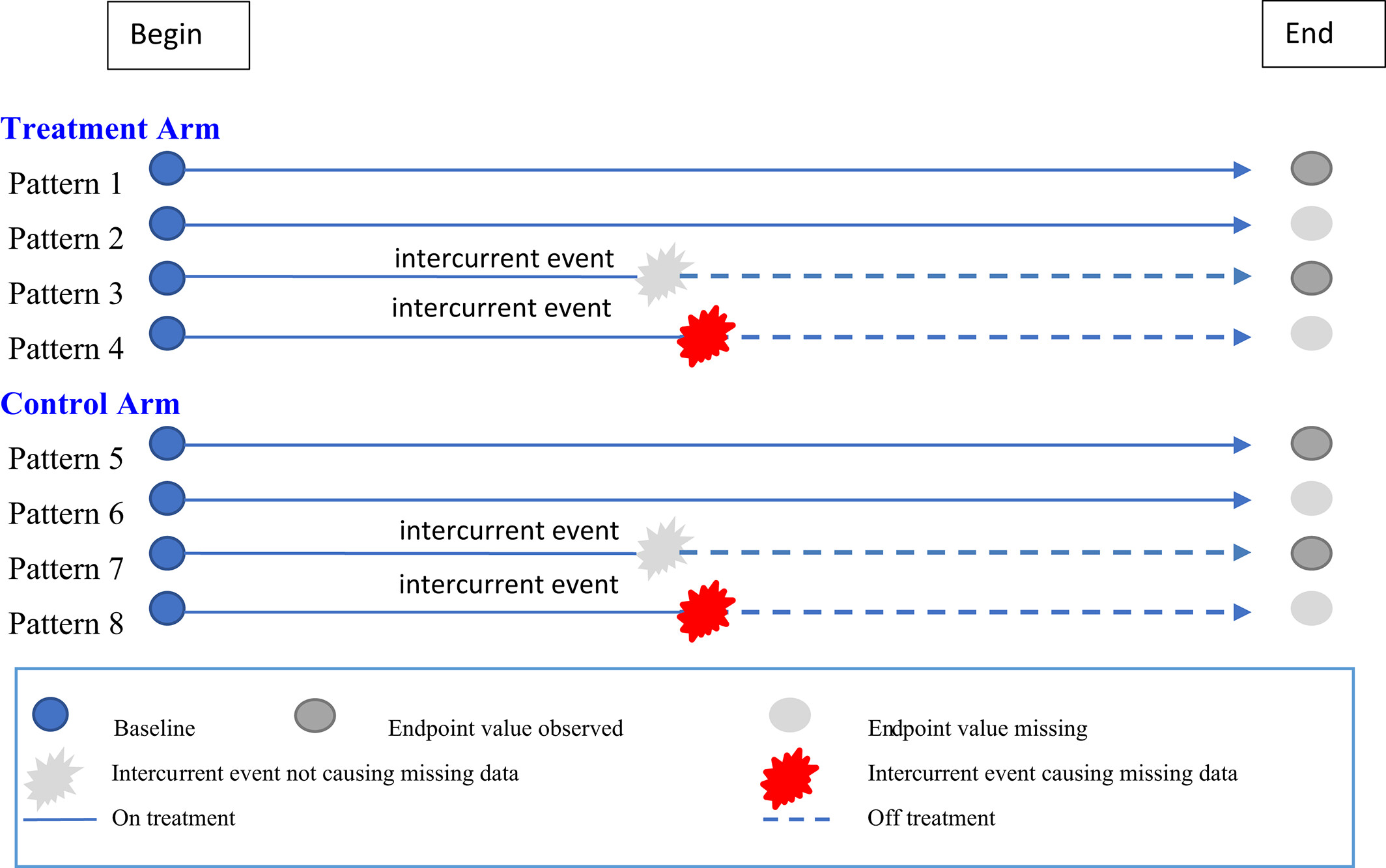
• Pattern 1 in the treatment arm and Pattern 5 in the control arm represent subjects who complete both the study treatments and the primary endpoint assessments (on-treatment completers).
• Pattern 2 in the treatment arm and Pattern 6 in the control arm represent subjects who complete the study treatments but miss the primary endpoint assessments (on-treatment incompleters).
• Pattern 3 in the treatment arm and Pattern 7 in the control arm represent subjects who experience intercurrent events, resulting in discontinuing or changing study treatments, but the subjects stay in the study and complete their primary endpoint assessments (retrieved dropouts (RDs)).
• Pattern 4 in the treatment arm and Pattern 8 in the control arm represent subjects who experience intercurrent events, resulting in discontinuing or changing study treatment, and the subjects drop out from the study and miss their primary endpoint assessments (non-retrieved dropouts (non-RDs)).

There should be very few subjects in Pattern 2 or 6. For such subjects, it may be reasonable to assume data are missing at random (MAR) and observed data from Patterns 1 and 5 can be used to impute missing data from Patterns 2 and 6, respectively. 

In this article, Wang et al. assumed that there are no subjects in Pattern 2 or 6 [Note: because these scenarios are rare in real world], and their focus is on imputing missing data from Patterns 4 and 8 that is, missing data occurring after and likely caused by intercurrent events. These data are very likely missing not at random. [Note: this is the missing data problems under treatment policy strategy]

Estimand used in the simulation study

Treatment	Experimental treatment versus placebo/active control
Target population	Adult subjects with type 2 diabetes mellitus (T2DM) inadequately controlled with diet and exercise alone or with background therapy
Variable of interest	Change in HbA1c from baseline to Week 26 (30 or 52)
Handling of intercurrent events	Treatment policy strategy is used in handling all intercurrent events: treatment discontinuation due to adverse event or lack of efficacy, use of rescue medication. All subjects should be followed up for the variable of interest and all data collected will be used in estimating the treatment effect regardless the occurrence of intercurrent events
Population-level summary	Difference in mean change in HbA1c from baseline between experimental and control arms

Statistical Methodology

Consider a longitudinal, randomized, parallel trial in which subjects receive either an experimental treatment (Exp) or a control treatment (Ctr).

Observed and missing data

Let \(Y = [y_1, y_2, y_3, \dots, y_{J-1}, y_J]\) be an \(n\) by \(J\) matrix, where each column vector \(y_j = [y_{j,1}, y_{j,2}, \dots, y_{j,i}, \dots, y_{j,n-1}, y_{j,n}]^T\) records a continuous endpoint of interest (e.g., HbA1c in a diabetes trial) measured from \(n\) subjects at a pre-specified timepoint \(j\), for \(j = 1, \dots, J-1, J\). Specifically, \(y_1\) and \(y_J\) are the measurements taken at baseline and the primary timepoint of interest (e.g., HbA1c at Week 26), respectively.

In practice, \(y_1\) can be completely observed, but missing records in \(y_J\) are unavoidable.

Consider \(y_J = (y_J^{(obs)}, y_J^{(mis)})\), a partition of \(y_J\) into two parts consisting of the observed data \(y_J^{(obs)}\) and the missing data \(y_J^{(mis)}\).

Missing data imputation under bayesian paradigm

By specifying a complete data model for \(y_J = P(y_J | \theta^*)\), an imputation model developed under a Bayesian paradigm can be generally described as the following two-step procedure:

• (a) Simulate a random draw of the unknown parameter \(\theta^*\) from the observed-data posterior: \[\tilde{\theta} \sim P(\theta^* | y_J^{(obs)})\]

• (b) Simulate a random draw of the missing values from the conditional predictive distribution: \[\tilde{y}_J^{(mis)} \sim P(y_J^{(mis)} | \tilde{\theta}, y_J^{(obs)})\]

With some vague prior on the model parameter \(\theta^*\), the implementation of Step (b) is often straightforward. On the other hand, the observed-data posterior \(P(\theta^* | y_J^{(obs)})\) in Step (a) does not always assume an analytic form, and thus may require additional statistical techniques (e.g., data augmentation) to simulate the desired stationary distributions.

Note: in short, we need data augmentation to simulate stationary distributions without explicit analytic forms. Data Augmentation is a technique where the computer “guesses” the missing data to help refine the parameters, then uses those parameters to refine the guesses.

During Imputation Step (I-Step): The model makes an educated “guess” to fill in the missing values based on the currently estimated patterns in the observed data.

During Posterior Step (P-Step): It treats those “guessed” values as if they were real data and recalculates the overall model rules (parameters).

This process repeats thousands of times until the guesses and the rules stop changing significantly. This “stationary distribution” provides the most statistically probable values for the missing data, even without a simple analytical equation.

In some cases when the complete data model \(P(y_J | \theta^*)\) assumes a special form, the analytic expression of \(P(\theta^* | y_J^{(obs)})\) does exist, and the two-step procedure can be readily applied by making sequential draws as specified in Steps (a) and (b). A case in point is a linear regression model for \(y_J\) (or some transformation thereof) parameterized by \(\theta^* = (\beta, \sigma^2)\), that is, \(P(y_J | X, \beta, \sigma^2) = N(X\beta, \sigma^2)\), where \(X\) is a covariate matrix consisting of variables that are correlated with \(y_J\) and/or plausibly affect the missingness of \(y_J\), \(\beta\) is the corresponding regression coefficient vector, and \(\sigma^2\) is the residual variance. Under this model assumption, \(P(\theta^* | y_J^{(obs)})\), or specifically, \(P(\beta | X, y_J^{(obs)})\) and \(P(\sigma^2 | X, y_J^{(obs)})\) are the posterior predictive distributions of the parameters in the linear regression built based on the observed data, and can be easily expressed as a function of a standard normal distribution and a chi-square distribution, respectively.（Note: when \(Y \sim\) normal distribution, the elegance of its mathematical characteristics stems from the existence of closed-form analytic expressions）

However, the complete truth about this underlying data structure is hardly known, due to information loss caused by missing data. Thus, plausible assumptions about missing data (e.g., the mechanisms of missingness) are needed prior to the development of an imputation model (Note: more details about different assumptions can be made when using different imputation approaches like Return2Baseline/J2R/CR/MMRM…).

RDO approach

As subjects from both groups discontinue their assigned treatments due to intercurrent events, it is reasonable to assume that RDs and non-RDs from the same treatment arm share similar clinical outcomes, after adjustment of baseline covariates (denoted as X).

With enough RDs, missing data in non-RDs could be addressed, to the best of our knowledge, as how the measurement would have been, had it been measured.

Missing data in an endpoint for non-RDs (Patterns 4 and 8, figure above) can be imputed based on the observed data from the RDs in the same treatment arm (i.e., Patterns 3 and 7 respectively).

Denote \(Y_{RD}^{(obs)}\) as the observed data from RDs in Pattern 3. The conditional predictive distribution to be used in imputing missing data in non-RDs in Pattern 4 is

\[ P(Y_{J}^{(mis)} \mid \theta^{*},Y_{RD}^{(obs)},X) \] A similar model can be used to impute missing data from non-RDs in Pattern 8 based on observed data from RDs in Pattern 7.

How about intermediate missing? In both models, besides baseline data, intermediate observed data can be used from both RDs and non-RDs. If some scheduled intermediate assessments are missing, they can be imputed first assuming MAR to create a monotone missing pattern before imputing \(P(Y_{J}^{(mis)})\).

Algorithm

Once the data from RDs are selected for the MI, the following steps can be used to impute missing data:

1. Intermediate missing data points are imputed using Markov Chain Monte Carlo (MCMC) to give a monotone missing data pattern. This step can be repeated N \(\ge\) 100 times to give N datasets. [Note: The MCMC imputation model in Step 1 should only include continuous covariates, considering that it is based on a multivariate normal distribution. Instead of change from baseline, Wang et al. recommended using absolute measurements at scheduled visits in the imputation models, so that occasional subjects with missing baseline values but with post-baseline values may still be included.]

2. For each of the N datasets in Step 1, create 2 subsets:

Subset 1: subjects classified as off-treatment at the endpoint visit. These subjects are either RDs or non-RDs. I.e., This includes the Retrieved Dropouts (people who stopped meds but gave data) AND the Non-RDs (people who stopped meds and gave no data)

Subset 2: on-treatment completers. I.e., people who stayed on meds and finished the trial.

3. Within each Subset 1 from Step 2, perform monotone regression imputation once for those with missing data to give one complete subset.

4. Combine each of the completed subsets from Step 3 with the on-treatment completers (Subset 2) to give one complete dataset.

5. Apply an Analysis of Covariance (ANCOVA) model with the pre-specified covariates (for example, the most commonly used model for analyzing HbA1c change from baseline in a diabetes trial) on each of the N complete datasets to calculate the estimates and standard errors of least square (LS) means and treatment differences.

6. Use Rubin’s rules6 to combine and synthesize N sets of results from Step 5 to estimate an overall treatment effect and corresponding variability.

If SAS is used to implement the above procedures, in Step 5, the OBSMARGINS or the om option for LS means should be included in the PROC MIXED SAS procedure whenever there are class covariates in the model in addition to treatment, such as randomization strata and country. With this option, the LS means will be adjusted according to the baseline distribution of the covariates. Otherwise, equal weights will be assigned to each category of the categorical covariate.

The RD approach is the authors’ preferred method for imputing missing data resulting from intercurrent events.

However, with limited sample size of RDs, a convergence problem may arise if there are many covariates in the imputation model. If convergence problem persists even with a minimal model structure, other imputation methods, such as the return to baseline (RTB) method or the washout method etc., should be considered.

/* Step 1: MCMC to create Monotone Missing Pattern */
/* Note: Only continuous covariates included as per recommendation */

proc mi data=adlb out=mi_mcmc 
        nimpute=100      /* N >= 100 datasets */
        seed=12345;      /* Set seed for reproducibility */
    
    /* Using MCMC to impute intermittent missing data to force a monotone pattern */
    /* chain=multiple ensures independence between imputations */
    mcmc chain=multiple impute=monotone;
    
    /* VAR statement order matters: usually Baseline -> Visit 1 -> Visit 2 -> Visit 3 */
    var base aval1 aval2 aval3; 
run;

/* Step 2: Define Subsets */
data subset_off_tx subset_completers;
    set mi_mcmc;
    
    /* Subset 1: Off-treatment (RDs and Dropouts) */
    /* This group contains the missing data we want to impute using RD logic */
    if status = 'OFF_TX' then output subset_off_tx;
    
    /* Subset 2: On-treatment Completers */
    /* These subjects are fully observed and need no further imputation */
    else output subset_completers;
run;

/* Step 3: Impute Missing Data in Subset 1 using Monotone Regression */
/* Since the input is only 'OFF_TX', the model parameters are derived solely from RDs */

proc mi data=subset_off_tx out=subset_off_tx_filled 
        nimpute=1 /* We already have 100 datasets; we just fill the missingness in each existing one */
        seed=67890;
    
    /* Crucial: Process each of the 100 datasets independently */
    by _Imputation_; 
    
    /* Step 3 specifies Monotone Regression */
    monotone reg(aval3 = base aval1 aval2); 
    
    var base aval1 aval2 aval3;
run;

/* Step 4: Combine the imputed Subset 1 with the static Subset 2 */
data final_imputed;
    set subset_off_tx_filled subset_completers;
    
    /* Sort to ensure tidy organization for the next step */
    by _Imputation_ usubjid; 
run;

/* Step 5: Run ANCOVA on each imputed dataset */

proc mixed data=final_imputed;
    by _Imputation_; /* Run the model 100 times */
    
    class trt strata;
    
    /* Standard ANCOVA Model: Change = Baseline + Treatment + Strata */
    /* Note: If modeling absolute value, target is AVAL3. If change, create CHG variable first */
    model aval3 = base trt strata / s; 
    
    /* LSMEANS with OBSMARGINS (om) */
    /* This weights the means by the observed covariate distribution */
    lsmeans trt / diff om cl; 
    
    /* Save the LSMeans and Differences to datasets for pooling */
    ods output Diffs=mixed_diffs LSMeans=mixed_lsm;
run;

/* Step 6: Synthesize results using Rubin's Rules */

/* Sort is required before MIANALYZE */
proc sort data=mixed_diffs; by trt _trt; run;

proc mianalyze data=mixed_diffs;
    /* Define the categorization of the difference (e.g., Drug vs Placebo) */
    class trt _trt; 
    
    /* The variable containing the treatment difference estimate */
    modeleffects estimate; 
    
    /* The variable containing the Standard Error of that estimate */
    stderr stderr; 
run;

Simulation setup

For simulation purposes, the dataset consisting solely of trial completers serves as the starting point. From the completers’ dataset, a two-step procedure (the selection step followed by the replacement step) is implemented to synthesize different scenarios of treatment discontinuation. In the selection step, a subgroup of subjects is selected from the completers’ dataset and marked as “discontinued from treatment.” In the replacement step, the Week 26 HbA1c measurement of each selected subject is replaced by a new value simulated to reflect the impact of treatment discontinuation on the treatment effect. Details of the two-step procedure follow.

Note:以由completers组成的数据集作为起点——从该completers数据集中，采用两步——先“选择步骤”，后“替换步骤”，来“合成”不同的treatment discontinuation情景。在“选择步骤”中，从completers数据集中选出一组受试者，并将其标记为“治疗中断”。在“替换步骤中”，每位被选受试者第26周的HbA1c测量值将被一个新值取代——该新值通过模拟生成，以反映治疗中断对治疗效果的影响。大概思路还是常规的模拟方式——先生成完整的observed data，再挖空

Scenario 1: The Random Quitters (MCAR) The Logic: Discontinuation Completely at Random.

Roll a die: It doesn’t matter if the patient is doing great or failing miserably; everyone has an equal chance of dropping out. E.g., a patient moves to a different city or changes jobs and can’t make appointments. It has nothing to do with the drug.

Scenario 2: “The Curse of Competence” (Discontinuation due to Adverse Events)

This scenario assumes that if a drug is very potent, it might work too well. Patients who have the massive drops in HbA1c (the “Top Performers”) might also be getting the highest exposure to the drug, leading to side effects (Adverse Events or AEs). [Note: 药效过强 \(\rightarrow\) AE]

How to pick them: Rank everyone by how much their HbA1c dropped \(\rightarrow\) Look at the “Top Performers” (e.g., the top \((k+10) \%\)) \(\rightarrow\) Randomly select the \(k\%\) dropouts from that top group.

This is dangerous - If we delete the “best” patients, the remaining drug arm looks worse than it actually is.

Scenario 3: “Quitting While Behind” (Discontinuation due to lack of Efficacy [LOE])

This is common in the Placebo Arm. Patients taking the placebo notice they aren’t getting better. Frustrated by the “Lack of Efficacy” (LOE), they quit the trial. The patients in the Placebo Arm who had the worst improvement (or got worse) may got CUT.

How to pick them: Rank everyone \(\rightarrow\) Look at the \((k+10) \%\) “Bottom Performers” (those with zero change or rising HbA1c) \(\rightarrow\) Randomly select \(k \%\) dropouts from that bottom group

If we delete the “worst” placebo patients, the remaining placebo arm looks better than it actually is.

Scenario 4: The Real World (Mixture: Discontinuation due to adverse event or lack of efficacy)

This combines Scenarios 2 and 3.

Treatment Arm: Loses the “Best” patients (due to side effects).

Placebo Arm: Loses the “Worst” patients (due to lack of effect).

Result: This is the “Worst Case Scenario” for proving a drug works. We are artificially lowering the average of the drug arm and raising the average of the placebo arm, narrowing the gap between them.

How to do it mathematically?

In each scenario described above, the observed Week 26 HbA1c of a selected subject will be replaced by a new simulated value. Specifically, for Subject \(i\) who discontinues treatment, let \(y_{i,1}^{\text{Obs}}\) and \(y_{i,26}^{\text{Obs}}\) denote the subject’s observed baseline and Week 26 measurements from the completers’ dataset, respectively. A new Week 26 HbA1c measurement \(y_{i,26}^{\text{Sim}}\) is simulated based on one of two settings:

\[ y_{i,26}^{\text{Sim}} \sim N \left(\mu_i, \sigma \right), \quad \text{with } \mu_i = y_{i,26}^{\text{Obs}} + \left| \left( y_{i,26}^{\text{Obs}} - y_{i,1}^{\text{Obs}} \right) \right| \times \left(1 - R_f \right), \tag{1} \]

\[ y_{i,26}^{\text{Sim}} \sim N \left(\mu_i, \sigma \right), \quad \mu_i = y_{i,26}^{\text{Obs}} - \left| E_C \right| \times B_f. \tag{2} \]

In both settings, \(y_{i,26}^{\text{Sim}}\) is generated from a normal distribution, centered at \(y_{i,26}^{\text{Obs}}\) plus a shift, and perturbed by a noise level of \(\sigma\) (which is set to the residual standard deviation estimated from the MMRM model based on the completers’ data in our simulation). Setting 1 simulates the situation in which subjects have worse glycemic level after treatment discontinuation than if they stay on treatment. In this setting, \(y_{i,26}^{\text{Sim}}\) is expected to be greater than \(y_{i,26}^{\text{Obs}}\) by an assumed margin of \(\left| \left( y_{i,26}^{\text{Obs}} - y_{i,1}^{\text{Obs}} \right) \right| \times \left(1 - R_f \right)\), where \(R_f\) (or the retention factor) is a percentage that ranges between 0% and 100% and dictates how much treatment effect is retained from the previously assigned treatment. When \(R_f = 100\%\), \(\mu_i = y_{i,26}^{\text{Obs}}\), implying that the treatment effect is retained 100%. The retained treatment effect diminishes as \(R_f\) decreases. Setting 2 simulates the situation that subjects have improved glycemic control after treatment discontinuation than if they stay on treatment. In this setting, \(y_{i,26}^{\text{Sim}}\) is expected to be less than \(y_{i,26}^{\text{Obs}}\) by an assumed margin of \(\left| E_C \right| \times B_f\), where \(E_C\) is the overall placebo-adjusted treatment effect estimated from the MMRM model based on the completers’ dataset, and \(B_f\) (or the benefit factor) is a percentage that specifies the amount of treatment benefit regained after treatment discontinuation due to possible benefit from rescue therapy. When \(B_f = 100\%\), \(\mu_i = y_{i,26}^{\text{Obs}} - \left| E_C \right|\), suggesting that the subject enjoys full treatment benefit after treatment discontinuation. The treatment benefit dwindles as \(B_f\) decreases.

Because the treatment effect is expected to taper off after subjects withdraw from the active treatment, Setting 1 is applied in Scenarios 1 through 4 to simulate \(y_{i,26}^{\text{Sim}}\) for the discontinued subjects in the experimental arm. Additionally, considering a possible diminution of the placebo effect after placebo treatment discontinuation, Setting 1 is also applied to generate \(y_{i,26}^{\text{Sim}}\) for discontinued subjects in the placebo arms in Scenarios 1 and 2. Finally, in Scenarios 3 and 4, Setting 2 is applied to simulate \(y_{i,26}^{\text{Sim}}\) for subjects who discontinue from the placebo treatment. For these two scenarios, treatment discontinuation is due to lack of efficacy, and subjects are expected to gain some treatment benefit from available rescue medications (table below).

Replacement step settings applied to simulate for the discontinued subjects in Scenarios 1–4 from the selection step.

	Scenario 1	Scenario 2	Scenario 3	Scenario 4
Experimental arm	Setting 1	Setting 1	Setting 1	Setting 1
Placebo arm	Setting 1	Setting 1	Setting 2	Setting 2

Upon completion of the two-step procedure, we simulate a complete dataset, which we will refer to as our truth dataset. The real treatment effect \(E_R\) and its standard error \(S_R\) are set to the LSmean treatment difference and its standard error estimated from an ANCOVA performed based on the truth dataset. This ANCOVA model used change in HbA1c at Week 26 from baseline as the dependent variable and treatment and other baseline covariates as independent variables.

For each truth dataset simulated above, the discontinued subjects are further divided into two categories: the RDs and subjects with missing primary outcomes (or the non-RDs). Specifically, we randomly select a fraction of discontinued subjects as RDs. For the non-RDs, discard their \(y_{i,26}^{Sim}\) values and set their endpoint measurements as missing.

Comparisons of statistical methods for missing data imputation?

These following two statistics serve as convenient metrics to evaluate the accuracy and efficiency of the estimates resulted from different imputation methods (Note: this paper compares five MI methods via Markov Chain Monte Carlo simulations and showcases how three of these five methods have been applied to estimate the treatment effects published in the labels for three antihyperglycemic agents currently on the market).

• \(E_I, S_I\): treatment effect, standard error for method I.

• \(E_R, S_R\): treatment effect, standard error for real data set.

Bias is defined as \(E_R-E_I\).

Variability inflation is defined as \(S_I/S_R\).

========Read the origin paper for the results of simulations=======

Discussion

Executive Summary: Managing Data and Intercurrent Events

The paper emphasizes that while intercurrent events (such as treatment intolerance) are inevitable, they should not be conflated with missing data. The authors argue that valid results depend on both preventing missing data and utilizing appropriate statistical methods.

Key Recommendations for IND Review To minimize missing data, drug applicants are advised to take three specific actions:

• Investigator Training: Educate site investigators on the critical nature of subject retention.

• Subject Education: Update consent forms to explain why data collection remains scientifically vital even if the patient discontinues the treatment early.

• Active Retention: Implement logistical support (e.g., transportation offers, contacting family) to maintain contact with subjects who are difficult to reach.

Outcomes and Statistical Validity

• Success in Antihyperglycemic Trials: By adopting these communication strategies and targeting a “treatment policy estimand,” recent NDAs for antihyperglycemic products have successfully reduced missing data rates to less than 5%.

• Methodological Rigor: Low missing data rates alone are insufficient. The primary efficacy analysis must still use valid statistical methods that target an estimand strictly aligned with the study’s specific objectives.

For statistical analysis methodology

Primary Methods for Handling Missing Data

The authors outline approaches (not mentioned above) to handling missing data under the treatment policy estimand, specifically within the context of Type 2 Diabetes Mellitus (T2DM) trials (excluding Type 1 Diabetes/insulin).

• Preferred Method (RD-based): Model missing measurements of non-Retrieved Dropouts (non-RDs) based on known measurements from Retrieved Dropouts (RDs) within the same treatment group.
• Alternative Methods: When there are insufficient RDs to model from, two specific methods are recommended based on the study type:
• Washout Method: For placebo-controlled studies.
• Return-to-Baseline (RTB) Method: For active-controlled studies.

Validation and Sensitivity Analysis

Since all imputation relies on untestable assumptions, the authors emphasize the necessity of Sensitivity Analysis to test the robustness of the primary results.

• Alignment: Sensitivity analyses must target the same estimand as the primary analysis. (e.g., An RTB analysis is a valid check for a Washout primary analysis, but an MMRM analysis is not).

• Tipping-Point Analysis: This method involves systematically varying imputed data to identify scenarios where statistical significance is lost. Results are considered robust only if significance is lost in scenarios unlikely to occur in reality.

Warning: One cannot simply add penalties to a “Missing At Random” (MAR) model; the tipping point must be based on an appropriate primary analysis.

• Non-Inferiority Studies: Special care is required here. Methods like RTB and Washout can be conservative and attenuate treatment differences, potentially falsely indicating non-inferiority.

Solution: Imputation should be performed under the non-inferiority null hypothesis, potentially by penalizing the experimental group by the non-inferiority margin.

Scope and Future Research

While the current research focuses on continuous endpoints in antihyperglycemic development, the methods are extensible:

• Time-to-Event Endpoints: The RD approach has been applied here, though analysts must use “proper” imputation (Type A) if using Rubin’s rules to avoid underestimating variance.

• Count & Categorical Endpoints: The authors have recommended the RD method for these endpoints during IND reviews but have not yet applied them in NDA/BLA reviews. This remains a key area for future research.

Reference

Bell, J., Drury, T., Mütze, T., Pipper, C. B., Guizzaro, L., Mitroiu, M., & Wright, D. (2025). Estimation methods for estimands using the treatment policy strategy; a simulation study based on the PIONEER 1 trial. Pharmaceutical Statistics, 24(2), e2472.

Carpenter, J. R., Roger, J. H., & Kenward, M. G. (2013). Analysis of longitudinal trials with protocol deviation: A framework for relevant, accessible assumptions, and inference via multiple imputation. Journal of Biopharmaceutical Statistics, 23(6), 1352–1371.

Cro, S., Carpenter, J. R., & Kenward, M. G. (2019). Information-anchored sensitivity analysis: Theory and application. Journal of the Royal Statistical Society Series A: Statistics in Society, 182(2), 623–645.

Polverejan, E., & Dragalin, V. (2020). Aligning treatment policy estimands and estimators—A simulation study in Alzheimer’s disease. Statistics in Biopharmaceutical Research, 12(2), 142–154.

Roger, J. H., Bratton, D. J., Mayer, B., Abellan, J. J., & Keene, O. N. (2019). Treatment policy estimands for recurrent event data using data collected after cessation of randomised treatment. Pharmaceutical Statistics, 18(1), 85–95.

Sabanes Bove, D., Dedic, J., Kelkhoff, D., Kunzmann, K., Lang, B., Li, L., Wang, Y. (2022). mmrm: Mixed Models for Repeated Measures. R package version 0.2.2, <https:// CRAN.R-project.org/package=mmrm>

Wang, Y., Tu, W., Kim, Y., Sinks, S., He, J., Cambon, A., & Clark, J. (2023). Statistical methods for handling missing data to align with treatment policy strategy. Pharmaceutical Statistics, 22, 650.

White, I., Joseph, R., & Best, N. (2020). A causal modelling framework for reference-based imputation and tipping point analysis in clinical trials with quantitative outcome. Journal of Biopharmaceutical Statistics, 30(2), 334–350.