Reference-based Multiple Imputation (3) - Algorithm of J2R
Estimand
De Jure Estimand
For response profile \(\mathbf{Y}\), and any suitable function \(g(\cdot)\), \(\tilde{f}_{act}\) as joint prob distribution function of baseline and post-randomization reponses for patients randomized to active treatment (\(f_{cont}\) for control group), we define the de jure estimand as
\[ \mathrm{E}_{\tilde{f}_{act}}[g(\mathbf{Y})] - \mathrm{E}_{\tilde{f}_{cont}}[g(\mathbf{Y})]. \tag{1} \]
De Facto Estimand
For response profile \(\mathbf{Y}\), and any suitable function \(g(\cdot)\), we define the de facto estimand as
\[ \mathrm{E}_{{f_{act}}}[g(\mathbf{Y})] - \mathrm{E}_{{f_{cont}}}[g(\mathbf{Y})]. \tag{2} \]
Mathematics setup
Consider a randomized clinical trial with two treatment arms, baseline and continuous longitudinal follow-up.
Let \(i = 1, \dots, n\) index patients
Let \(j = 0, \dots, J\) index the \(J\) scheduled observation times, with \(j = 0\) denoting baseline.
Let \(T_i\) denote randomized arm.
Let \(Y_{ij}\) denote the response at time \(j\) for subject \(i\).
For simplicity, assume there are no interim missing data and all patients are observed at baseline.
For each subject, let \(D_i\) now denote the last observation time prior to a deviation
Note: … or ICE. This paper was published before ICH E9 R1
Since we assume everyone was observed at baseline, \(D_i\) can take values \(0, \dots, J\).
Very often post-deviation responses will be missing; otherwise for this exposition we set them to missing.
The approach falls in the pattern mixture framework (Little, 1993; Kenward and Carpenter, 2009).
Note:
The authors mention their approach falls under the “pattern mixture framework.” Instead of assuming one giant model for everyone, this method groups patients by their “pattern” of missingness (typically, the exact time they dropped out, \(D_i\)).
It builds a different statistical model for each group, acknowledging that a patient who drops out on Day 10 (as an example) might have a fundamentally different clinical trajectory than someone who drops out on Day 100.
For each subject, let the column vector \(\mathbf{Y}_{Oi} = (Y_{i0}, \dots, Y_{iD_i})^T\) denote the subject’s observed responses, at times \(j = 0, \dots, D_i\), and, if \(D_i < J\).
Let the column vector \(\mathbf{Y}_{Mi} = (Y_{i(D_i+1)}, \dots, Y_{iJ})^T\) denote post-deviation responses at times \(D_i + 1, \dots, J\).
Let \(\mathbf{Y}_M\) be the column vector \((\mathbf{Y}_{M1}^T, \dots, \mathbf{Y}_{Mn}^T)^T\) and \(\mathbf{Y}_O\) be the column vector \((\mathbf{Y}_{O1}^T, \dots, \mathbf{Y}_{On}^T)^T\). [实际上这是多个患者组成的矩阵]
Note:
The data \(\mathbf{Y}_{Oi}\) collected before the patient deviated or dropped out (up to time \(D_i\)).
The data \(\mathbf{Y}_{Mi}\) that should have been collected after the patient deviated, but wasn’t.
The goal of the math in the text is to figure out the most statistically sound way to guess (impute) \(\mathbf{Y}_{Mi}\) based on \(\mathbf{Y}_{Oi}\) and the specific time they dropped out (\(D_i\)).
For each patient, the distribution of that person’s post-deviation responses, given that person’s pre-deviation responses and deviation time, is denoted
\[ [\mathbf{Y}_{Mi} \mid \mathbf{Y}_{Oi}, D_i, T_i, \boldsymbol{\eta}]. \tag{3} \]
Given a specific parametric form for equation (3) (typically multivariate normal), \(\boldsymbol{\eta}\) are the parameters of this distribution, whose values we have to estimate before we can impute missing post-deviation data by drawing from equation (3). [需要估计参数\(\eta\)之后,才能Impute missing data]
If data are MAR, then equation (3) does not depend on \(D_i\), and is simply \([\mathbf{Y}_{Mi} \mid \mathbf{Y}_{Oi}, T_i, \boldsymbol{\eta}]\).
Note: The fact that the data is missing can be completely explained by the data we already have. If the data is MAR, the text notes that the dropout time (\(D_i\)) doesn’t matter for the underlying math. We can predict the missing values just by looking at the patient’s past trajectory and treatment arm.
However, if post-deviation data are missing not at random (MNAR), this distribution will depend on \(D_i\), in a way that could be different for each individual.
The missingness is related to the missing data itself. For example, a patient stops showing up because their unrecorded symptoms are getting worse. If data is MNAR, we cannot just look at past data; the distribution of the missing data changes depending on exactly when and why they dropped out (\(D_i\)). 简单来说,缺失值与缺失机制有关.
Thus, for each individual, or more typically groups of individuals, we define a form for equation (3) that reflects a specific assumption appropriate to their treatment arm, deviation time, and possibly other relevant information.
Given this, we use multiple imputation for inference.
In essence, this works as follows.
Multiple imputation
Depending on the question at hand, let \(\theta\) denote the quantity defined by Estimand (1) or (2).
If no deviations occur relevant to the question, then we estimate this by \(\hat{\theta} = \hat{\theta}(\mathbf{Y})\).
Otherwise, \(\hat{\theta} = \hat{\theta}(\mathbf{Y}_M, \mathbf{Y}_O)\).
For inference about \(\theta\) in the presence of deviations, multiple imputation creates \(K\) “complete” data sets by:
MI1. Taking a draw from the Bayesian posterior distribution of \([\boldsymbol{\eta} \mid \mathbf{Y}_O]\) and then
MI2. Drawing the missing data from equation (3) using the above draw of \(\boldsymbol{\eta}\).
Both steps are repeated to create each imputed data set.
The parameter of interest is then estimated from each completed data set in turn to give \(\hat{\theta}_k\), with standard error \(\hat{\sigma}_k\), \(k = 1, \dots, K\).
These are then combined using Rubin’s rules (Rubin, 1987) to give a single multiple imputation estimate and associated standard error.
To implement MI1 we need to choose a model for the observed data, which specifies the parameters \(\boldsymbol{\eta}\). To implement MI2 we need to specify equation (3).
Taking the former first, given our setting of longitudinal response data measured at scheduled times, we choose an unstructured multivariate normal model, with a separate mean for each time point in each arm and a separate unstructured covariance matrix in each arm.
As there are two arms, \(\boldsymbol{\eta}\) consists of \(2 \times (J + 1)\) means [两组,基线与基线后] and \(2 \times \{(J + 1)(J + 2)/2\}\) variance/covariance parameters [参数分布在对角阵,有两组].
Before describing our proposal for the second step in detail, our generic approach is set out in subsection below (named “Generic Algorithm”).
Then another subsection describes in detail what seem to us—based on experience with these analyses and the regulatory authorities—five natural options for piecing together \([\mathbf{Y}_{Mi} \mid \mathbf{Y}_{Oi}, D_i, T_i, \boldsymbol{\eta}]\) (这篇博文我只看J2R).
Generic Algorithm
G1. Separately for each treatment arm, take all patients’ pre-deviation data and—assuming MAR—fit a multivariate normal distribution with unstructured mean (i.e., a separate mean for each of the \(1 + J\) baseline plus post-randomization observation times) and unstructured variance–covariance matrix (i.e., a \((1 + J) \times (1 + J)\) covariance matrix) using a Bayesian approach with an improper prior for the mean and an uninformative Jeffreys prior for the variance–covariance matrix (Schafer, 1997, p. 155).
G2. Separately for each treatment arm, draw a mean vector and variance–covariance matrix from the posterior distribution.
G3. For each patient who deviates before the end of the study, use the draws from step G2 to build the joint distribution of that patient’s pre- and post-deviation outcome data. Suggested options for constructing this are given in subsection.
G4. For each patient who deviates before the end, use that patient’s joint distribution in step G3 to construct the conditional distribution of post-deviation given pre-deviation outcome data. Sample the post-deviation data from this conditional distribution, to create a “completed” data set.
G5. Repeat steps G2–G4 \(K\) times, resulting in \(K\) imputed data sets.
G6. Fit the model of interest to each imputed data set, and combine the resulting parameter estimates and standard errors using Rubin’s rules Rubin (1987) for final inference.
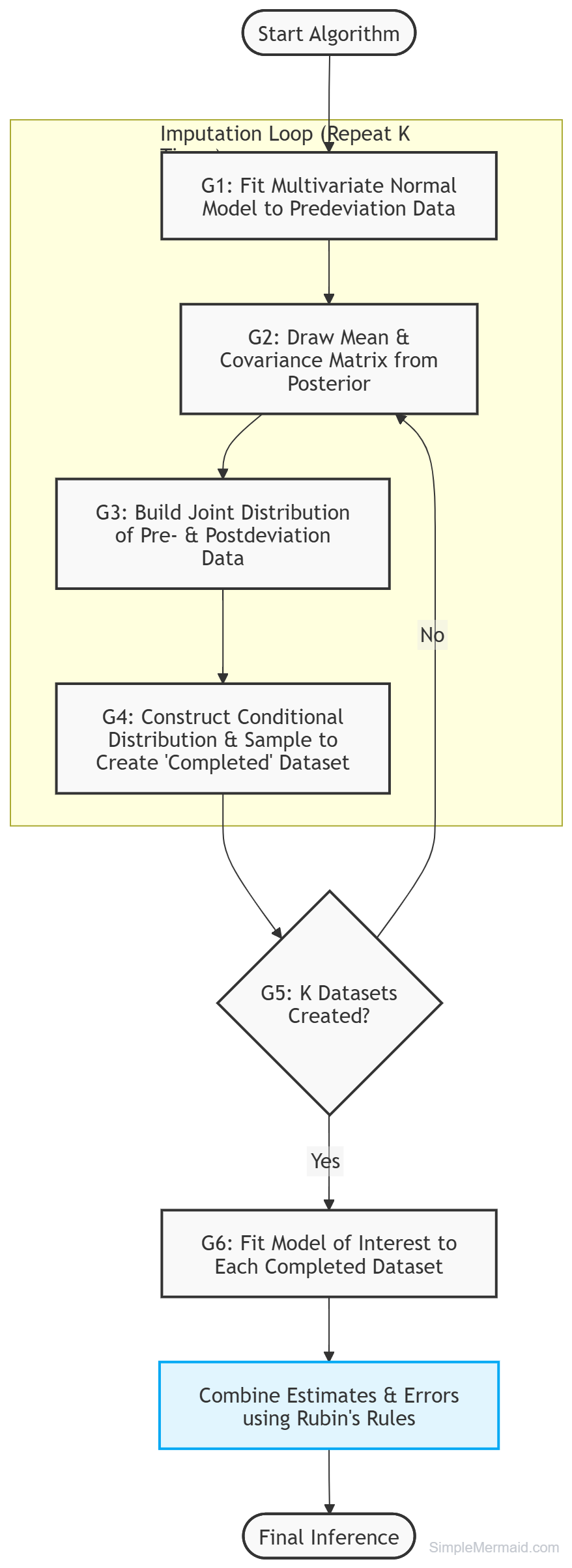
We use the Markov-Chain Monte Carlo method to sample from the appropriate Bayesian posterior in step G2, updating the chain sufficiently between successive draws to ensure draws are effectively independent.
Some Notes….
在J2R框架下,步骤 G1 和 G2 负责从现有的观察数据中提取统计特征,并为后续的随机插补提供参数。
G1: 拟合观测数据的模型 (Fitting the Model)
在这一步中,我们不考虑任何缺失数据,只看目前手里已有的、在发生偏倚前收集到的真实数据。
分层建模:算法要求分别对每个治疗组(试验组和参考组)进行操作。
多元正态分布 (MVN):我们假设患者的所有时间点数据(基线 + \(J\) 个随访点)服从一个多元正态分布。
非结构化参数 (Unstructured; UN):
- 均值向量:不假设随访曲线是直线还是曲线,而是为每个时间点都设定一个独立的平均值。
- 方差-协方差矩阵:不假设时间点之间的相关性是对称的或递减的,而是允许任意两个时间点之间都有独立的相关系数。
贝叶斯先验 (Bayesian Priors):为了后续能够进行“抽取”,这里使用了贝叶斯方法。
- 对均值使用Improper prior,对协方差矩阵使用Jeffreys prior。在看到数据之前,对参数一无所知,从而让最终结果完全由数据驱动。
G2: 从贝叶斯后验分布中抽取 (Drawing from the Posterior)
为什么不直接用 G1 算出来的平均值,而要Draw?
如果只用一个固定的平均值去预测缺失数据,就忽略了“我们对平均值的估算本身也是不确定”这一事实。
通过从后验分布中随机抽取 \(K\) 组参数(均值 \(\mu\) 和协方差 \(\Sigma\)),我们模拟了参数估计中的不确定性。
操作:
根据 G1 得到的数据分布,生成一个后验分布(即给定观察数据后,参数 \(\boldsymbol{\eta}\) 可能取值的概率分布)。
随机从这个分布中拿出一组 \(\mu\) 和 \(\Sigma\)。
这组抽取的参数将作为后续 G3 和 G4 步骤中生成缺失值的输入参数。
总结:
| 步骤 | 目标 | 类比 |
|---|---|---|
| G1 | 理解数据 | 观察参考组和试验组患者的过往表现,画出概率分布图。 |
| G2 | 模拟不确定性 | 并不是给出一个唯一的答案,而是从“可能的参数范围”里随机摇号,选出一组参数。 |
通过重复这个过程 \(K\) 次(通常 \(K=50\) 或 \(100\)),我们就能创建出多个略有不同的“完整数据集”,从而满足多重插补(Multiple Imputation)的要求。
Constructing Joint Distributions of Pre- and Post-deviation Outcome Data
We propose the following options for constructing the joint distribution of each patient’s pre- and post-deviation outcome data in step G3.
Each option represents a possible de jure or de facto assumption concerning post-deviation data.
Many others are possible, but these are sufficient to explain our approach and illustrate its flexibility.
Note: 此处我只选择review MAR与J2R
Randomized-arm MAR.
The joint distribution of the patient’s observed and post-deviation outcome data is multivariate normal with mean and covariance matrix from their randomized treatment arm.
Jump to reference.
Post deviation, the patient ceases randomized treatment, and patient’s mean response distribution is now that of a “reference” group of patients (typically, but not necessarily, control patients).
Such a change may be seen as extreme, and choosing the reference group to be the control group might be used as a worst-case scenario in terms of reducing any treatment effect since withdrawn patients on active will lose the effect of their period on treatment.
Post-deviation data in the reference arm are imputed under randomized-arm MAR.
Technical details for J2R
Here is a breakdown of the “Jump to Reference” assumption and the matrix math used to construct the new covariance matrix.
1. J2R Assumption Explained
In clinical trials, when a patient stops taking the experimental drug (deviates), we have to guess (impute) what their missing future data would have looked like.
The J2R assumption proposes a specific clinical scenario:
Before Dropout (\(t \le D_i\)): The patient was on the active drug, so their data follows the statistical profile (mean and variance) of the active arm.
After Dropout (\(t > D_i\)): The patient stopped the active drug.
J2R assumes that any beneficial effect of the experimental drug instantly vanishes.
From that point forward, the patient’s expected trajectory “jumps” to match the trajectory of the reference arm (usually the placebo or standard-of-care control group). 也就是说,post-deviation或者post-ICE,患者会jump to reference
Mathematically, their mean vector simply glues these two realities together: \[\tilde{\mu}_i = (\underbrace{\mu_{a,0}, \dots, \mu_{a,D_i}}_{\text{Active Arm Means}}, \underbrace{\mu_{r,D_i+1}, \dots, \mu_{r,J}}_{\text{Reference Arm Means}})^T\]
2. Breaking Down the Covariance Matrix (\(\widetilde{\Sigma}\))
While the mean vector is just glued together, the variance-covariance matrix is trickier.
We can’t just glue two matrices together because the resulting matrix might not be “positive definite” (a strict mathematical requirement for covariance matrices, ensuring variances are never negative). Furthermore, the future data must logically correlate with the past data.
We construct the new covariance matrix for these observations as follows.
Denote the covariance matrices from the reference arm (without deviation) and the other arm in question (without deviation) [Note: 这里矩阵是基于reference arm和active arm里without deviation的数构造的], partitioned at time \(D_i\) according to the pre- and post-deviation measurements (行与列都基于Di分割), by:
\[ \text{Reference } \Sigma_r = \begin{bmatrix} \mathbf{R}_{11} & \mathbf{R}_{12} \\ \mathbf{R}_{21} & \mathbf{R}_{22} \end{bmatrix} \quad \text{and other arm: } \quad \Sigma_a = \begin{bmatrix} \mathbf{A}_{11} & \mathbf{A}_{12} \\ \mathbf{A}_{21} & \mathbf{A}_{22} \end{bmatrix}. \]
We want the new covariance matrix, \(\widetilde{\Sigma}\) say, to match that from the active arm for the pre-deviation measurements, and the reference arm for the conditional components for the post-deviation given the pre-deviation measurements. This also guarantees positive definiteness of the new matrix, since \(\Sigma_r\) and \(\Sigma_a\) are positive definite. That is, we want
\[ \widetilde{\Sigma} = \begin{bmatrix} \widetilde{\Sigma}_{11} & \widetilde{\Sigma}_{12} \\ \widetilde{\Sigma}_{21} & \widetilde{\Sigma}_{22} \end{bmatrix}, \]
Note:
\(\widetilde{\Sigma}\)是这个方法非常核心的内容。他们试图为最初接受试验药物(active arm)但随后退出(deviate)的患者,构建一个新的混合统计分布模型,具体来说,是一个新的协方差矩阵,记作 \(\widetilde{\Sigma}\). 协方差矩阵的作用是描述患者的测量数据如何波动,以及不同时间点的测量值之间如何相互关联。这个新的协方差矩阵是没办法从原来基于MAR的模型里得到的。
“…match that from the active arm for the pre-deviation measurements…” 这个部分读起来比较直观。当患者还在按方案接受试验药物时(即退出试验之前),他们的身体对药物是有反应的。因此,描述他们Deviation/ICE发生之前的数学模型应该与试验组(active arm)的模型(即矩阵块 \(\mathbf{A}_{11}\))完美匹配。这里非常直观,我们知道他们\(D_i\)之前在用试验药,所以他们数据的方差就应该等于试验组的方差。
“…and the reference arm for the conditional components for the post-deviation given the pre-deviation measurements.” 这里比较难理解,以下是我自己的理解。强调conditional的原因,在我读起来,像是一旦患者退出,J2R假设认为他们会立刻失去试验药物的益处,并开始表现得像reference arm中的患者一样。
但是,我们又不能只简单粗暴地把reference arm未来的方差直接套用到这些患者身上。因为患者未来的健康状况与他们自己过去的健康状况是密不可分的。如果一个患者在第1、2、3周的某项指标一直很高,从数学概率上讲,无论他们突然改用什么治疗方法,他们在第4周的该项指标依然很可能偏高。在统计学中,基于我们已经掌握的过去信息来预测未来,需要依赖conditional distribution。
To solve this, the authors partition the covariance matrices into blocks based on the dropout time \(D_i\):
Block 11: Variance/covariance of the pre-deviation measurements.
Block 22: Variance/covariance of the post-deviation measurements.
Blocks 12 & 21: The correlation between the pre- and post-deviation measurements.
We have the active arm matrix (\(\Sigma_a\) made of \(\mathbf{A}\) blocks) and the reference matrix (\(\Sigma_r\) made of \(\mathbf{R}\) blocks). We need to build a hybrid matrix (\(\widetilde{\Sigma}\)) and now we have prepared well.
The Three Constraints (这里是三个限制条件,我们要基于以下等式求解出各个\(\widetilde{\Sigma}_{ij}\) [\(i=1,2;\quad j=1,2\)]):
The authors define three rules to build this hybrid matrix:
Constraint 1: The past is the past. The variance of the data collected before the patient dropped out must perfectly match the active treatment arm, because they were taking the active drug (见上述我的理解). \[\widetilde{\Sigma}_{11} = \mathbf{A}_{11} \tag{4}\]
Constraint 2: The relationship between past and future matches the reference group. In multivariate normal distributions, the matrix product \(\Sigma_{21}\Sigma_{11}^{-1}\) acts like the slope in a regression—it dictates how a change in the past (index 11) affects the future (index 21). Because the patient is now effectively in the reference group, this “slope” must match the reference arm’s slope. \[\widetilde{\Sigma}_{21}\widetilde{\Sigma}_{11}^{-1} = \mathbf{R}_{21}\mathbf{R}_{11}^{-1} \tag{5}\]
Constraint 3: The residual variance matches the reference group. When we predict the future based on the past, there is leftover uncertainty (residual variance). This complex-looking formula represents that conditional variance. Again, since the patient is now acting like a control patient, this leftover uncertainty must match the control arm’s uncertainty. \[\widetilde{\Sigma}_{22} - \widetilde{\Sigma}_{21}\widetilde{\Sigma}_{11}^{-1}\widetilde{\Sigma}_{12} = \mathbf{R}_{22} - \mathbf{R}_{21}\mathbf{R}_{11}^{-1}\mathbf{R}_{12} \tag{6}\]
The Solution (基于等式4,5,6,求解各个\(\widetilde{\Sigma}_{ij}\)):
By doing some matrix algebra and substituting equation (4) into (5), and then into (6), you arrive at the final formulas for the hybrid matrix blocks:
- \(\widetilde{\Sigma}_{11} = \mathbf{A}_{11}\) (Straightforward substitution).
- \(\widetilde{\Sigma}_{21} = \mathbf{R}_{21}\mathbf{R}_{11}^{-1}\mathbf{A}_{11}\) (Solving Constraint 2 for \(\widetilde{\Sigma}_{21}\)).
- \(\widetilde{\Sigma}_{22} = \mathbf{R}_{22} - \mathbf{R}_{21}\mathbf{R}_{11}^{-1}(\mathbf{R}_{11} - \mathbf{A}_{11})\mathbf{R}_{11}^{-1}\mathbf{R}_{12}\) (Solving Constraint 3 for \(\widetilde{\Sigma}_{22}\)).
3. Considerations in Implementation (最重要的部分)
The text notes something highly convenient at the very end.
When we actually go to impute the missing data using the conditional distribution, the math works out such that we don’t actually need to calculate this complex \(\widetilde{\Sigma}\) matrix.
We can just use the reference arm’s matrix (\(\mathbf{R}\)) directly for the imputation step (Step G4), saving significant computational power.
Note:
这里作者的意思是:
我们可以直接用reference arm的\(\mathbf{R}\)矩阵直接做G4的填补。
这确实非常反直觉,核心点在于:我们只插补“未来”(缺失的数据),我们不需要插补“过去”(已观察到的数据)。
理解这个问题的关键在于:多元正态分布的条件概率公式到底需要提取协方差矩阵里的哪些参数?
在步骤 G4 中,我们需要生成患者退出试验后缺失的数据(未来数据),而依据是他们退出前已经观察到的数据(过去数据)。
对于MVN分布,给定过去数据预测未来数据,核心只需要从协方差矩阵中提取并计算两个关键components:
斜率(回归系数): 决定了过去的数据表现会如何拉动对未来的预测:\(\Sigma_{21}\Sigma_{11}^{-1}\)
条件方差(残差): 决定了预测值周围还有多大的随机误差:\(\Sigma_{22} - \Sigma_{21}\Sigma_{11}^{-1}\Sigma_{12}\)
关键点: 插补未来缺失数据时,绝对不需要用到 \(\Sigma_{11}\) 本身(即过去数据自身的方差)。既然过去的数据已经是白纸黑字的确切记录(as-observed),我们不需要用算法去“猜”它,因此过去数据本该有多大的波动(\(\mathbf{A}_{11}\) 还是 \(\mathbf{R}_{11}\)),在生成未来随机数时根本用不上。
为什么作者说 \(\mathbf{R}\) 和 \(\widetilde{\Sigma}\) 算出的结果一模一样?
回看那个复杂的混合矩阵 \(\widetilde{\Sigma}\) 的求解约束条件:
- 约束条件 (5) 等式锁死了斜率: \[\widetilde{\Sigma}_{21}\widetilde{\Sigma}_{11}^{-1} = \mathbf{R}_{21}\mathbf{R}_{11}^{-1}\]
这条规则在数学上保证了:使用混合矩阵 \(\widetilde{\Sigma}\) 算出的预测斜率,完全等于直接使用参考组矩阵 \(\mathbf{R}\) 算出的斜率。
- 约束条件 (6)等式锁死了条件方差: \[\widetilde{\Sigma}_{22} - \widetilde{\Sigma}_{21}\widetilde{\Sigma}_{11}^{-1}\widetilde{\Sigma}_{12} = \mathbf{R}_{22} - \mathbf{R}_{21}\mathbf{R}_{11}^{-1}\mathbf{R}_{12}\]
这条规则在数学上保证了:使用混合矩阵 \(\widetilde{\Sigma}\) 算出的预测波动范围,也完全等于直接使用参考组矩阵 \(\mathbf{R}\) 算出的波动范围。
插补算法在底层生成缺失数据时,只会向协方差矩阵索要“斜率”和“条件方差”这两个组件 。
既然作者通过公式 (5) 和 (6) 在数学上强制规定了: \(\widetilde{\Sigma}\) 的 [斜率, 条件方差] 必须等价于 \(\mathbf{R}\) 的 [斜率, 条件方差]
那么,不管费尽心思拼接出的 \(\widetilde{\Sigma}\) 输入给插补软件,还是直接把现成的 \(\mathbf{R}\) 输入给软件,软件提取出来的核心参数是一模一样的,最终生成的插补值也就完全相同。
这个巧妙的数学shortcut允许在编程实现时走捷径:直接拿参考组的整个矩阵去跑插补算法,从而在不破坏“跳转到参考组”逻辑的前提下,大幅节省计算步骤。
4. SAS
Implementation: Scientific Working Group on Estimands and Missing Data: Five Macros
The macros must be run in sequence. They automatically share information between themselves so that no information needs to be specified more than once.
Part1A declares the parameter estimation model and checks consistency with the dataset. It builds a master dataset which holds details of the current job (run of the macros in sequence). It also builds indexes for the classification variables, which may be either numeric or character.
Part1B fits the parameter estimation model using the MCMC procedure and draws a pseudo-independent sample from the joint posterior distribution for the linear predictor parameters and the covariance parameters.
Part2A calculates the predicted mean under MAR, and under MNAR for each subject based on their withdrawal pattern once for each draw of the linear predictor parameter estimates. The choice of MNAR is controlled by the method used, which may vary from subject to subject.
Part2B imputes the intermediate missing values using MAR and the trailing missing values using MNAR, by deriving the conditional distribution for the missing values conditional on the observed values and covariates, using the appropriate sampled covariance parameter estimates.
Part3 carries out a univariate ANOVA analysis at selected time points usually based on the same covariates as the parameter estimation model. It then combines the least-squares means and their differences using the MIANALYZE procedure to provide final results. It is in this macro which handles the Delta methods. The macro parameters and their function are listed in a later section.
Core parts of the “five-macros”:
| Macro | Core Function | Statistical Output | Key SAS Procedure |
| Part1B | Learns the trial dynamics | Posterior Parameter Draws | PROC MCMC |
| Part2A | Calculates patient trajectories | Posterior Predictive Means | PROC FCMP |
| Part2B | Injects realistic variance | Posterior Predictive Samples | CALL CHOL / RAND |
Reference
Carpenter JR, Roger JH, Kenward MG. Analysis of longitudinal trials with protocol deviation: a framework for relevant, accessible assumptions, and inference via multiple imputation. J Biopharm Stat. 2013;23(6):1352-71. doi: 10.1080/10543406.2013.834911. PMID: 24138436.
Kenward , M. G. , Carpenter , J. R. ( 2009 ). Multiple imputation. In: A Handbook of Modern Statistical Methods. Davidian, M., Fitzmaurice, G., eds. Chichester, UK: Wiley, pp. 477–500 .
Little , R. J. A. ( 1993 ). Pattern mixture models for multivariate incomplete data . Journal of the American Statistical Association 88 : 125 – 134 .
Appendix - Notes on FiveMacros
Core parts of Part1B
Initial Estimates: Uses PROC MIXED to define the “unstructured” mean and covariance parameters (\(\boldsymbol{\eta}\)) that the MCMC will refine.
MCMC Sampling: This is Step G2, drawing \(K\) sets of parameters from the posterior distribution \([\boldsymbol{\eta} \mid \mathbf{Y}_O]\). PROC MCMC is strictly sampling the population-level model parameters. It is NOT sampling the estimated values for each individual subject.
Inside Part1B, PROC MCMC looks at all the observed data and samples the parameters (the “rules” of the trial). For each draw, it calculates:
The average effect of Treatment A at Visit 1, Visit 2, etc.
The average effect of Treatment B at Visit 1, Visit 2, etc.
The effect of the covariates (e.g., how much does age or weight shift the score?).
The variance-covariance matrix (how much natural bounce or noise is there between visits?).
Output Datasets: Creates the specific postLP and postCVP files that Step G4 requires to sample the missing post-deviation data.
/* =========================================================================
   CORE COMPONENT 1: Standardization & Data Preparation
   Centres and scales covariates to improve MCMC convergence for Step G1.
   ========================================================================= */
proc means data=&loc1A._datav noprint mean std;
    var &Cov &CovbyTime;
    output out=&jobname._mean mean= &Cov &CovbyTime;
    output out=&jobname._std std= &Cov &CovbyTime;
run;

/* Convert to Parallel (Wide) format and identify missing data patterns */
data &jobname._datap;
    merge &jobname._temp7 &jobname._temp12;
    by &subject;
    /* Logic to determine Super_Pattern (binary representation of missingness) */
    ...
run;

/* =========================================================================
   CORE COMPONENT 2: Initial Estimates for Priors (Step G1)
   Fits an unstructured MVN model to get starting values for the MCMC.
   ========================================================================= */
ods output solutionf=&jobname._Solf Covparms=&jobname._Covp;
proc mixed data=&jobname._data&DSver.;
    class &Subject I_&Treat I_&Time;
    model &Response = I_&Treat*I_&Time &STD_Cov / SOLUTION NOINT;
    repeated I_&time / SUBJECT=&Subject TYPE=UN Group=I_&Covgroup;
run;

/* =========================================================================
   CORE COMPONENT 3: The Bayesian Posterior Engine (Step G2)
   The actual PROC MCMC that draws parameters from the distribution.
   ========================================================================= */
proc mcmc data=dummy outpost=&jobname._classout
          nmc=%eval(&Ndraws * &thin) nbi=1000 thin=&thin jointmodel;

    BEGINCNST;
        /* Load clinical data into memory for likelihood calculation */
        rc = read_array("&jobname._datamcmc", Super_Response ...);
        ...
    ENDCNST;

    /* Define PRIORS (G1: Bayesian approach with improper/Jeffreys priors) */
    /* Means: Flat Prior */
    prior P_I_&Treat._1-P_I_&Treat._&Ntt ~ general(1);

    /* Covariance: Wishart Prior (requires sampling from chi-square) */
    prior W_LS&i ~ expchisq(%eval(&df-&j+1));
    prior W_Z ~ normal(0, var=1);

    /* LIKELIHOOD Calculation: Comparing observed data to the current draw */
    ll = 0;
    do s = 1 to &NSubj;
        nv = Ndata[p]; /* Number of visits for this pattern */
        /* Calculate Mu for the specific draw */
        Mu[i] = P_I_&Treat[it, time] + Covpart[s, time];
        /* Calculate the log-likelihood for this subject */
        mvnlp = logmpdfnormal(of Resp1-Resp&ii, of Mu1-mu&ii, "V"||Vpoint);
        ll = ll + mvnlp;
    end;

    model general(ll);
run;

/* =========================================================================
   CORE COMPONENT 4: Saving the Posterior Draws
   Reshaping MCMC output into parameter sets for the next Imputation step.
   ========================================================================= */
data &jobname._postLP; /* Saves Means/Linear Predictors */
    set &jobname._classout;
    /* Outputs one row per draw, per treatment, per timepoint */
    ...
run;

data &jobname._postCVP; /* Saves Covariance Matrices */
    set &jobname._classout;
    keep draw iteration RMVOUT_1-RMVOUT_...;
run;
Core parts of Part2A
The true “core” of this reference-based imputation (RBI) macro boils down to just two parts: The Mathematical Definitions of the Methods and The Posterior Draw Execution Loop.
This macro takes the “rules” found in Part1B and applies your specific Missing Not at Random (MNAR) assumptions (like Jump to Reference) to every individual patient who dropped out.
What it does: It acts as a deterministic calculator. For each of the 1,000 draws, it looks at a specific patient, calculates where they would have been under their assigned treatment, and then alters that trajectory based on when they dropped out and what method (J2R, CIR, CR, etc.) you requested.
The Math: It calculates the exact predictive mean (\(\hat{\mu}\)) for the missing timepoints. It does not add any random noise.
The Output: * _datapm: A massive dataset containing the exact calculated expected values for every patient, for every missing timepoint, across all 1,000 draws.
It should be noted that:
When Part1B finishes, it gives you 1,000 different “draws” of the trial’s parameters (treatment effects, covariate effects).
For a single subject (let’s say Patient #101), Part2A loops through all 1,000 of those draws and calculates their exact expected score.
Draw 1 says Patient #101’s mean should be 45.2
Draw 2 says Patient #101’s mean should be 45.6
Draw 3 says Patient #101’s mean should be 44.9
…and so on.
So, for Patient #101, Part2A creates a distribution of 1,000 expected means. This distribution represents our uncertainty about the true parameters (often called epistemic uncertainty). It reflects how confident the model is about where the “center” of the data should be.
Part2A gives you the distribution of the Predictive Means per subject (reflecting parameter uncertainty).
Part2B takes those means, adds the random variance/noise, and finally generates the true Posterior Predictive Distribution per subject.
The Imputation Formulas (proc fcmp)
This is the mathematical heart of the macro. It defines exactly how the missing values are calculated based on the treatment mean (This), the reference mean (Ref), and subject-specific covariates (MyCov).
proc fcmp outlib=work.funcs.trial;

* 1. Missing at Random (MAR);
function MAR(CausalK,Last,This[*],Ref[*],MyCov[*],Out[*]) $ 128;
    outargs This,ref,Out,Mycov;
    do i=1 to dim(out);
        out[i]=This[i]+Mycov[i];
    end;
    return("");
endsub;

* 2. Copy Increment from Reference (CIR);
function CIR(CausalK,Last,This[*],Ref[*],MyCov[*],Out[*]) $ 128;
    outargs This,ref,Out,Mycov;
    if last=0 then do;
        do i=1 to dim(out); out[i]=Ref[i]+Mycov[i]; end;
        return("No valid data. Increment is zero.");
    end;
    else do;
        do i=1 to last; out[i]=This[i]+Mycov[i]; end;
        do i=last+1 to dim(out);
            out[i]=Ref[i]-ref[last]+this[last]+Mycov[i]; /* Applies reference trajectory */
        end;
        return("");
    end;
endsub;

* 3. Jump to Reference (J2R);
function J2R(CausalK,Last,This[*],Ref[*],MyCov[*],Out[*]) $ 128;
    outargs This,ref,Out,Mycov;
    do i=1 to last; out[i]=this[i]+Mycov[i]; end;
    do i=last+1 to dim(out);
        out[i]=Ref[i]+Mycov[i]; /* Directly adopts reference mean */
    end;
    return("");
endsub;

* 4. Copy Reference (CR);
function CR(CausalK,Last,This[*],Ref[*],MyCov[*],Out[*])  $ 128;
    outargs This,ref,Out,Mycov;
    do i=1 to dim(out);
        out[i]=ref[i]+Mycov[i]; /* Assumes reference mean from the start */
    end;
    return("");
endsub;

* 5. Causal Model;
function CAUSAL(CausalK,Last,This[*],Ref[*],MyCov[*],Out[*]) $ 128;
    outargs This,ref,Out,Mycov;
    if last=0 then do;
        do i=1 to dim(out); out[i]=Ref[i]+Mycov[i]; end;
        return("No valid data.");
    end;
    else do;
        do i=1 to last; out[i]=This[i]+Mycov[i]; end;
        do i=last+1 to dim(out);
            /* Applies a user-defined proportional shift based on CausalK */
            out[i]=Ref[i]+ CausalK*(this[last]- ref[last])+Mycov[i];
        end;
        return("");
    end;
endsub;

/* Note: Other MCF (Mean Carried Forward) methods like OLMCF, ALMCF follow a similar structure */
quit;
The Posterior Execution Loop
This block inside the main data &jobname._datapm; step is where the macro actually applies the drawn posterior parameters to individual patients.
* Loop through every posterior draw;
do draw=1 to &Ndraws;
    do itime=1 to &Ntimes;

        * A[itime]: Predicted mean for the treatment arm at this timepoint;
        A[itime] = values[draw,I_&treat,itime] + AvgMeanp[draw,itime];

        * B[itime]: Predicted mean for the reference arm at this timepoint;
        if I_ref>.z then B[itime] = values[draw,I_Ref,itime] + AvgMeanp[draw,itime];
        else B[itime] = .;

        * MyCov[itime]: The subject-specific deviation from the average subject (covariate effects);
        MyCov[itime] = (0 &calc) - AvgMeanp[draw,itime];
    end;

    * Dynamically apply the chosen reference-based imputation method;
    select(Super_Method);
        when("MAR")    warntxt = MAR(Super_k, Super_Last, A, B, Mycov, C);
        when("CIR")    warntxt = CIR(Super_k, Super_Last, A, B, Mycov, C);
        when("J2R")    warntxt = J2R(Super_k, Super_Last, A, B, Mycov, C);
        when("CR")     warntxt = CR(Super_k, Super_Last, A, B, Mycov, C);
        when("CAUSAL") warntxt = CAUSAL(Super_k, Super_Last, A, B, Mycov, C);
        /* ... other methods ... */
    end;

    * Store the final imputed array (C) back into the dataset variables;
    do itime=1 to &Ntimes;
        super_mean[itime] = C[itime];
        super_mar[itime]  = A[itime] + MyCov[itime];
    end;

    output; * Write the draw to the final dataset;
end;
For J2R, Part 1 of the above code (While the patient is still in the trial): For i=1 up to the last observed timepoint, the output (Out[i]) is calculated using the Treatment mean (This[i]) plus the patient’s personal covariate adjustment (MyCov[i]).
Part 2 (After the patient drops out): Starting at last + 1 until the end of the trial, the macro completely abandons the treatment mean. It “jumps” to using the Reference mean (Ref[i]) plus their personal covariate adjustment (MyCov[i]).
Core parts of Part2B
This Part2b macro is the final assembly line. It takes the “expected averages” (the predictive means) calculated in Part2A, mixes them with the “expected variance” (the covariance matrices) from Part1B, and injects random statistical noise to generate the final, realistic imputed patient records.
The Missing Piece: The simulate Function At the very top of the code, in the PROC FCMP block, the author defines a subroutine called simulate. This is the random number generator we were looking for in the previous step.
subroutine simulate(a[*,*],b[*]);
    outargs a,b;
    /* ... setup ... */

    /* 1. Decompose the Covariance Matrix (a) using Cholesky Decomposition */
    call chol(a,chol);

    /* 2. Draw a standard normal random variable for each missing timepoint */
    do i=1 to n;
        normal[i]=rand('NORMAL');
    end;

    /* 3. Multiply the random variables by the Cholesky matrix to scale the noise correctly */
    call mult(chol,normal,b);
endsub;
What this does mathematically:
If you want to draw a random sample from a multivariate normal distribution with a specific covariance matrix (\(\Sigma\)), the standard statistical trick is to:
Draw a vector of completely independent, standard random numbers (\(z \sim N(0, I)\)).
Take the Cholesky decomposition of your covariance matrix (\(L\), where \(LL^T = \Sigma\)).
Multiply them together (\(Lz\)).
The output array b (which is later called simres) now contains the perfectly scaled and correlated random residual errors for the missing timepoints.
Imputing Intermediate Missing Values (Assuming MAR)
Before looking at the final dropouts, the macro first handles “intermediate” missing values (e.g., a patient missed Visit 2, but came back for Visit 3 and 4).
It does this inside a loop (%do Nmiss=1 %to %eval(&Ntimes-1);).
Because the patient came back, it is standard practice to assume the missed visit was Missing at Random (MAR). It uses conditional multivariate normal math to calculate the offset, taking into account the data observed before and after the missed visit.
/* s11: Covariance of observed times
   s12: Covariance between observed and missing times
   s22: Covariance of missing times */

call myinv(s11,invs11);
call mymult(invs11,s12,iS11S12);

/* Calculates how much the patient's observed data shifts their expected missing data */
call mymult(diff_1,iS11S12,offset);

/* Calculates the remaining unexplained variance for the missing timepoint */
call mysubtract(s22,S21iS11S12,ss22);

/* Draws the random noise based on that remaining variance */
call simulate(SS22,simres);

/* Final Imputed Value = Random Noise + Observed Offset + MAR Predictive Mean */
kkk = simres[i] + offset[1,i] + super_mar[point[&Nwith+i]];
Imputing Trailing Missing Values (Using MNAR Assumptions)
Once the intermediate holes are filled, it tackles the final dropouts. This is where the decisions made in Part2A (like J2R, CIR, or Causal) finally come into play.
Depending on the VCMethod requested (THIS, REF, or ZERO), the macro grabs the appropriate covariance matrix:
THIS: Uses the variance of the treatment the patient was actually on.
REF: Uses the variance of the Reference arm (standard for J2R).
It then performs the same conditional math as above: it calculates how the patient’s observed early data affects their expected later data (offset), calculates the remaining variance (ss22), and draws the random noise (simres).
/* Generates the correlated random noise for the remaining missing visits */
call simulate(ss22,simres);

do i=1 to &Ni;
    /* Final Imputed Value =
       Noise (simres) +
       Observed offset +
       The MNAR predictive mean calculated in Part2A (super_mean) */

    super_response[i+&Nwith] = simres[i] + offset[1,i] + super_mean[i+&Nwith];
end;
The Output: _DataFull
After looping through every patient, for every one of the 1,000 parameter draws, it outputs a dataset called &jobname._dataFull.
This is the final deliverable of the entire macro suite. If you asked for 1,000 draws, this dataset contains 1,000 perfectly complete, separate copies of your clinical trial data, ready to be analyzed by standard statistical procedures (like PROC MIXED and PROC MIANALYZE) to get the final robust standard errors and p-values.