Missing Data and EM Algorithm

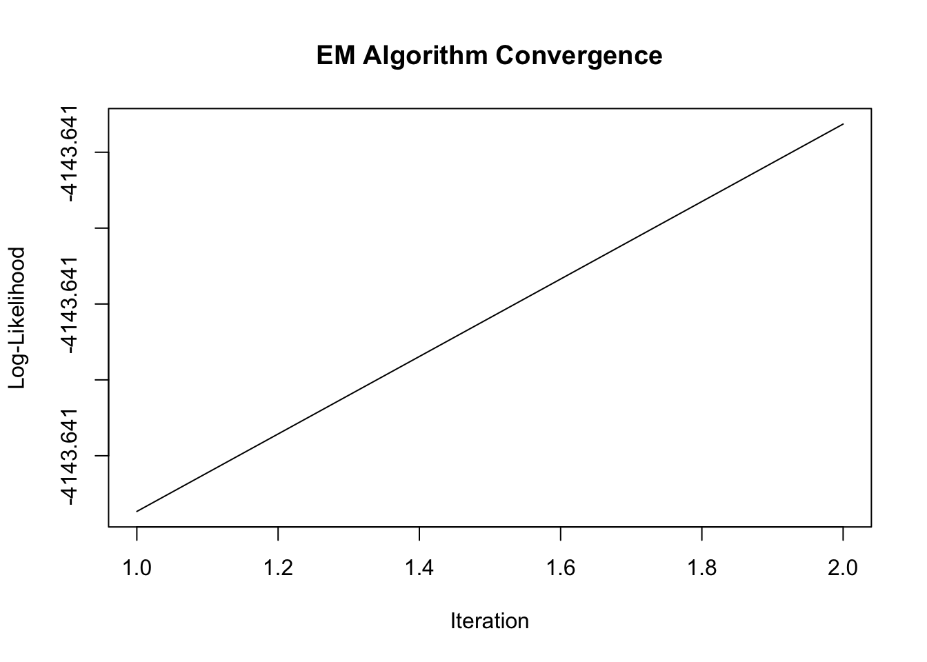
The expectation-maximization algorithm is an approach in which values of the statistics which would be computed if a complete dataset were available are estimated (imputed), taking into account the pattern of missing data.

Notation for Missingness

Data matrix \(Y\), missing data matrix \(M=\left \{M_{ij} \right \}\).

\[ M_{ij} = \left\{ \begin{array}{cl} 1 & : Y_{ij} \quad \text{is missing} \\ 0 & : Y_{ij} \quad \text{is observed} \end{array} \right. \]

Convenient to introduce the notation \(Y = (Yobs,Y_{miss})\), where \(Y_{miss}\) are conceptual and denote the data that were not observed.

Technical Categories of Patterns of Missingness

Abbreviations: S-Sex. R-Race. A-Admission. D-Department.

Univariate: \(M_{ij}=0\) unless \(j=j^*\).

Multivariate: \(M_{ij}=0\) unless \(j \in J \subset V\) (in my understanding, \(V\) is the set of variables). Example: For some subjects, both R and S unobserved.

Monotone: There is an ordering of \(V\) so \(M_{ik} = 0\) implies \(M_{ij} = 0\) for \(j < k\), e.g. drop-out in longitudinal studies. Example: For some, A is unobserved, others neither A nor R, but data otherwise complete.

Disjoint: Two subsets of variables never observed together. Controversial. Appears in Rubin’s causal model. Example: S and R never both observed.

General: none of the above. Haphazardly scattered missing values. Example: R unobserved for some, A unobserved for others, S,D for some.

Latent: A certain variable is never observed. Maybe it is even unobservable. Example: S never observed, but believed to be important for explaining the data.

Methods for Dealing with Missing Data

Complete case analysis: analyse only cases where all variables are observed.

Weighting methods. For example, if a population total \(\mu = E(Y)\) should be estimated and unit \(i\) has been selected with probability \(π_i\) a standard method is the Horwitz–Thompson estimator.

Imputation methods: Find ways of estimating the values of the unobserved values as \(Y_{miss}\), then proceed as if there were complete data. Without care, this can give misleading results, in particular because the ”sample size” can be grossly overestimated.

Model-based likelihood methods: Model the missing data mechanism and then proceed to make a proper likelihood-based analysis, either via the method of maximum-likelihood or using Bayesian methods. This appears to be the most sensible way. Typically this approach was not computationally feasible in the past, but modern algorithms and computers have changed things completely. Ironically, the efficient algorithms are indeed based upon imputation of missing values, but with proper corrections resulting.

Mechanisms of Missingness

MCAR

\[P(M = 1 | Y_{obs}, Y_{miss}) = P(M = 1)\]

Interpretation: The probability that data is missing is independent of both observed and unobserved data. The missingness is completely random and unrelated to any variables in the dataset.

Example: Example is recording error, latent variables, and variables that are missing by design (e.g. measuring certain values only for the first m out of n cases). Beware: it may be counterintuitive that missing by design is MCAR.

MAR

\[P(M = 1 | Y_{obs}, Y_{miss}) = P(M = 1 | Y_{obs})\]

Interpretation: The probability of missingness depends only on the observed data, not on the missing values themselves. Given the observed data, the missingness is random.

Example: Heuristically, only the observed values of \(Y\) have influence on the missingness. By design, e.g. if individuals with certain characteristics of \(Y_{obs}\) are not included in part of study (where \(Y_{miss}\) is measured).

Alternative notation:

\[P(M | Y_{obs}, Y_{miss}, \phi) = P(M | Y_{obs}, \phi)\]

where \(\phi\) represents parameters governing the missingness mechanism.

Note that if data are MCAR, they are also MAR.

MNAR

\[P(M = 1 | Y_{obs}, Y_{miss}) \neq P(M = 1 | Y_{obs})\]

or more explicitly:

\[P(M = 1 | Y_{obs}, Y_{miss}) = P(M = 1 | Y_{obs}, Y_{miss}, \phi)\]

Interpretation: The probability of missingness depends on the unobserved (missing) values themselves, even after accounting for observed data. This is the most challenging scenario.

Example: In an income survey, people with very high or very low incomes may be less likely to report their earnings, and this missingness depends on the actual (unobserved) income value. Another example will be: for example, if certain values of \(Y\) cannot be recorded when they are out of range, e.g. in survival analysis (censoring is another kind of missing data).

Summary

Mechanism	Depends on \(Y_{obs}\)	Depends on \(Y_{miss}\)	Bias in Complete Case Analysis
MCAR	No	No	No (but loss of efficiency)
MAR	Yes	No	Potentially Yes
MNAR	Yes	Yes	Yes

• MCAR: Complete case analysis is unbiased but inefficient. Simple methods like list-wise deletion are acceptable.

• MAR: Multiple imputation and maximum likelihood methods can produce unbiased estimates if the model is correctly specified.

• MNAR: Requires sensitivity analysis and specialized models. Assumptions about the missingness mechanism must be made explicit.

# Simulate data with different missing mechanisms
set.seed(123)
n <- 1000

# Complete data - from model y=2+3x+resid 
x <- rnorm(n)
y <- 2 + 3*x + rnorm(n)

# MCAR: 20% missing completely at random
y_mcar <- y
missing_mcar <- sample(1:n, size = 0.2*n)
y_mcar[missing_mcar] <- NA

# MAR: missingness depends on x
prob_mar <- plogis(-1 + 1.5*x)  # Higher x increases missing probability
missing_mar <- rbinom(n, 1, prob_mar) == 1
y_mar <- y
y_mar[missing_mar] <- NA

# MNAR: missingness depends on y itself
prob_mnar <- plogis(-1 + 0.5*y)  # Higher y increases missing probability
missing_mnar <- rbinom(n, 1, prob_mnar) == 1
y_mnar <- y
y_mnar[missing_mnar] <- NA

# Summary
cat("Proportion missing:\n")

Proportion missing:

cat("MCAR:", mean(is.na(y_mcar)), "\n")

MCAR: 0.2 

cat("MAR:", mean(is.na(y_mar)), "\n")

MAR: 0.323 

cat("MNAR:", mean(is.na(y_mnar)), "\n")

MNAR: 0.5 

Likelihood-based Methods

Complete Data and Observed Data Likelihood

Joint Likelihood: The complete data likelihood can be factored as:

\[L(\theta, \phi | Y, M) = f(Y, M | \theta, \phi) = f(Y | \theta) \cdot f(M | Y, \phi)\]

or written as \(L(\theta, \phi | Y, M) = P(Y, M | \theta, \phi) = P(Y | \theta) \cdot P(M | Y, \phi)\).

where:

• \(\theta\): parameters of the data model

• \(\phi\): parameters of the missingness model

The data likelihood \(P(Y_{obs}, Y_{miss} | \theta)\). The missingness probability \(P(M | Y_{obs}, Y_{miss}, \phi)\)

Ignorability Condition

The missing data mechanism is ignorable for likelihood-based inference if the following two conditions hold:

1. MAR: \(P(M | Y_{obs}, Y_{miss}, \phi) = P(M | Y_{obs}, \phi)\)
2. Parameter Distinctness: \(\theta\) and \(\phi\) are distinct (parameter spaces are separable [意义在于可直接相乘，进而分解Likelihood (separable)。见以下“Under Ignorability”章节。进一步的理解是，Joint parameter space of \((\theta,\phi)\) 必须可以分解为两个独立的parameter spaces的Cartesian Product，即\(\text{for }\theta \in \Theta \text{ and } \phi \in \Phi:\) 有\((\theta,\phi)\in \Theta \times \Phi\)]).

For the 2nd condition: the parameters \(\theta\) (for the data model) and \(\phi\) (for the missing mechanism) are distinct—knowing \(\theta\) tells us nothing about \(\phi\), and vice versa…

When both conditions hold, we can ignore the missing data mechanism and still make valid likelihood-based inferences about \(\theta\).

Implication

Under ignorability, the likelihood can be written as:

\[L(\theta | Y_{obs}, M) \propto P(Y_{obs} | \theta) \cdot P(M | Y_{obs}, \phi)\]

Since we’re only interested in \(\theta\), we can ignore the missingness mechanism and work with [因为distinctness,我们可以最大化\(\theta\)的似然函数，而不用考虑missing data]:

\[L(\theta | Y_{obs}) \propto P(Y_{obs} | \theta)\]

Maximum Likelihood Estimation (MLE)

The Full Likelihood

The complete likelihood for both the data and the missingness mechanism is:

\[ L(\theta, \phi | Y_{obs}, M) = \int P(Y_{obs}, Y_{miss} | \theta) \cdot P(M | Y_{obs}, Y_{miss}, \phi) \, dY_{miss} \] (see Appendix 1 for derivations…)

This is complex because:

• We must integrate over all possible values of missing data

• We must model the missingness mechanism.

Under Ignorability

When ignorability holds, we can factor the likelihood under distinctness:

\[L(\theta, \phi | Y_{obs}, M) = P(\theta | Y_{obs}) \times P(\phi | M, Y_{obs})\]

This is powerful because:

1. The first term \(L(\theta | Y_{obs})\) involves only the observed data likelihood
2. The second term \(L(\phi | M, Y_{obs})\) is about the missingness mechanism
3. They are separate - we can maximize them independently

Observed Data Likelihood

The observed data likelihood is obtained by integrating over the missing data:

\[ L(\theta | Y_{obs}) = \int P(Y_{obs}, Y_{miss} | \theta) dY_{miss} \]

Approach	Advantage	Disadvantage
Full Likelihood	Handles any missingness mechanism (including MNAR)	Must correctly specify the missingness model; more complex
Observed Likelihood	Simpler; no need to model missingness	Only valid under ignorability (MAR)

Full likelihood = Model the data + Model why data is missing

Observed likelihood = Model only the data we see

Under ignorability, both give valid inference for \(\theta\), so we can use the simpler observed likelihood.

The EM Algorithm for Missing Data

1. The Problem

The goal: We want to find the maximum likelihood estimate of \(\theta \in \Theta\) given observed data:

\[ \hat{\theta} = \arg\max_{\theta} P(\theta | Y_{obs}) = \arg\max_{\theta} P(Y_{obs} | \theta)=\arg\max_{\theta} \int P(Y_{obs}, Y_{miss} | \theta) \, dY_{miss} \]

The challenge: Direct maximization of the observed data likelihood is difficult because:

\[P(Y_{obs} | \theta) = \int P(Y_{obs}, Y_{miss} | \theta) \, dY_{miss}\]

This integral often has no closed form, making direct optimization intractable.

The solution: The EM algorithm iteratively maximizes a more tractable quantity.

2. The Q-Function

Since we don’t know \(Y_{miss}\), we take the expected value of the complete data log-likelihood, where the expectation is over the conditional distribution of \(Y_{miss}\) given \(Y_{obs}\) and current parameter estimate \(\theta^{(t)}\).

Define the Q-function - the expectation of complete data log-likelihood:

\[Q(\theta | \theta^{(t)}) := E \left[ \log P(Y_{obs}, Y_{miss} | \theta) \mid Y_{obs}, \theta^{(t)} \right]\]

\[= \int \log P(Y_{obs}, Y_{miss} | \theta) \cdot P(Y_{miss} | Y_{obs}, \theta^{(t)}) \, dY_{miss}\]

• Use current guess \(\theta^{(t)}\) to infer a distribution over missing values

• Average the complete data log-likelihood over this distribution

• Then maximize with respect to \(\theta\)

3. The EM Algorithm

Starting from an initial guess \(\theta^{(0)}\), iterate:

E-Step (Expectation)

Compute the expected complete data log-likelihood given observed data and current parameters:

\[Q(\theta | \theta^{(t)}) = E \left[ \log P(Y_{obs}, Y_{miss} | \theta) \mid Y_{obs}, \theta^{(t)} \right]\]

This requires computing (or characterizing) the conditional distribution, NOT the marginal distribution \(P(Y_{miss}\mid \theta^{(t)})\):

\[P(Y_{miss} | Y_{obs}, \theta^{(t)})\]

M-Step (Maximization)

Find the parameter value that maximizes the Q-function:

\[\theta^{(t+1)} = \arg\max_{\theta} Q(\theta | \theta^{(t)})\]

Iteration

Repeat E-step and M-step until convergence:

\[|\theta^{(t+1)} - \theta^{(t)}| < \epsilon \quad \text{or} \quad |\ell(\theta^{(t+1)}) - \ell(\theta^{(t)})| < \epsilon\]

4. Why EM Works: Theoretical Justification

The Observed Log-Likelihood Decomposition

We can decompose the observed log-likelihood as:

\[\ell(\theta) = \log P(Y_{obs} | \theta)\]

Using \(P(Y_{obs}) = \frac{P(Y_{obs}, Y_{miss})}{P(Y_{miss} | Y_{obs})}\):

\[\log P(Y_{obs} | \theta) = \log P(Y_{obs}, Y_{miss} | \theta) - \log P(Y_{miss} | Y_{obs}, \theta)\]

Taking expectations with respect to \(P(Y_{miss} | Y_{obs}, \theta^{(t)})\):

\[\ell(\theta) = Q(\theta | \theta^{(t)}) - H(\theta | \theta^{(t)})\]

Where:

\[H(\theta | \theta^{(t)}) = E_{Y_{miss} | Y_{obs}, \theta^{(t)}} \left[ \log P(Y_{miss} | Y_{obs}, \theta) \right]\]

Key Inequality

By Gibbs’ inequality (or Jensen’s inequality):

\[H(\theta | \theta^{(t)}) \leq H(\theta^{(t)} | \theta^{(t)})\]

with equality when \(\theta = \theta^{(t)}\).

Proposition - Ascent property of the EM

The EM iterations satisfy:

\[ \ell(\theta^{(t+1)}) \geq \ell(\theta^{(t)}) \]

Proof:

\[\ell(\theta^{(t+1)}) - \ell(\theta^{(t)}) = \underbrace{\left[Q(\theta^{(t+1)} | \theta^{(t)}) - Q(\theta^{(t)} | \theta^{(t)})\right]}_{\geq 0 \text{ by M-step}} - \underbrace{\left[H(\theta^{(t+1)} | \theta^{(t)}) - H(\theta^{(t)} | \theta^{(t)})\right]}_{\leq 0 \text{ by Gibbs}}\]

Both terms are non-negative, so \(\ell(\theta^{(t+1)}) \geq \ell(\theta^{(t)})\).

Theorem - Convergence property of the EM

Under some conditions, the sequence \(\{ \theta^{(t)} \}\) defined by the EM iterations converges to a stationary point of the observed data log-likelihood.

5. EM for Exponential Families

When the complete data distribution belongs to an exponential family, EM simplifies beautifully.

Exponential Family Form

\[P(Y_{obs}, Y_{miss} | \theta) = h(Y_{obs}, Y_{miss}) \exp\left[\eta(\theta)^T T(Y_{obs}, Y_{miss}) - A(\theta)\right]\]

Where:

• \(T(Y_{obs}, Y_{miss})\) = sufficient statistics

• \(\eta(\theta)\) = natural parameters

• \(A(\theta)\) = log-partition function

The log of this integral destroys the nice exponential family structure:

\[\log P(Y_{obs} | \theta) = \log \int \exp[\eta(\theta)^T T(Y_{obs}, Y_{miss}) - A(\theta)] \, dY_{miss}\]

Log of integral = hard to optimize! The Solution: Complete Data Model

The complete data log-likelihood is simple:

\[\log P(Y_{obs}, Y_{miss} | \theta) = \eta(\theta)^T T(Y_{obs}, Y_{miss}) - A(\theta) + \text{const}\]

No integral inside the log = easy to optimize! 总结起来，observed data likelihood需要解积分，使得优化非常复杂。而complete data likelihood没有积分形式，相对来说会更容易优化。

Complete Data Log-Likelihood

\[\log P(Y_{obs}, Y_{miss} | \theta) = \log h(Y_{obs}, Y_{miss}) + \eta(\theta)^T T(Y_{obs}, Y_{miss}) - A(\theta)\]

Instead of computing: \[T(Y_{obs}, Y_{miss}) \quad \text{← Can't do this! We don't have } Y_{miss}\]

We compute: \[\hat{T}^{(t)} = E[T(Y_{obs}, Y_{miss})| Y_{obs}, \theta^{(t)}]\]

We can’t calculate the sufficient statistics from complete data. So we calculate the average sufficient statistics across all possible values the missing data could be. This average is weighted by how likely each value is given what we observe.

Q-Function

\[Q(\theta | \theta^{(t)}) = \text{const} + \eta(\theta)^T E[T(Y_{obs}, Y_{miss})| Y_{obs}, \theta^{(t)}] - A(\theta)\]

E-Step Simplification

For exponential families, the E-step reduces to computing (或者用estimating更贴切) the complete-data sufficient statistics by:

\[\hat{T}^{(t)} = E[T(Y_{obs}, Y_{miss})|Y_{obs}, \theta^{(t)}]\]

The expected sufficient statistics.

M-Step Simplification

The M-step is the same as complete-data MLE, but using \(\hat{T}^{(t)}\) instead of the observed sufficient statistics.

Once we have \(\hat{T}^{(t)}\), we maximize as if it came from complete data (即可显示地去求解\(\theta\)):

\[\theta^{(t+1)} = \arg\max_{\theta} \left[\eta(\theta)^T \hat{T}^{(t)} - A(\theta)\right]\]

This is exactly the same as the complete data MLE, except we use \(\hat{T}^{(t)}\) instead of \(T(Y)\).

Comments: from the above E-step and M-step, in such cases, the computational problem is effectively confined to the E-step, which involves estimating (or “imputing”) the statistics \(T(Y)\), using the step shown in E-Step Simplification.

6. Concrete Example: Univariate Normal with Missing Data

Setup

• \(Y_i \stackrel{iid}{\sim} N(\mu, \sigma^2)\) for \(i = 1, \ldots, n\)
• \(Y_{obs} = \{Y_i : M_i = 0\}\) with \(n_{obs}\) observations
• \(Y_{miss} = \{Y_i : M_i = 1\}\) with \(n_{miss}\) missing values
• Assume MAR (ignorable missingness)
• Parameters: \(\theta = (\mu, \sigma^2)\)

Complete Data Log-Likelihood

\[\ell_c(\mu, \sigma^2) = -\frac{n}{2}\log(2\pi\sigma^2) - \frac{1}{2\sigma^2}\sum_{i=1}^{n}(Y_i - \mu)^2\]

Sufficient Statistics

\[T_1 = \sum_{i=1}^{n} Y_i, \quad T_2 = \sum_{i=1}^{n} Y_i^2\]

We can write: \[T_1 = \sum_{i: M_i=0} Y_i + \sum_{i: M_i=1} Y_i = T_1^{obs} + T_1^{miss}\]

\[T_2 = \sum_{i: M_i=0} Y_i^2 + \sum_{i: M_i=1} Y_i^2 = T_2^{obs} + T_2^{miss}\]

E-Step

Under \(P(Y_{miss} | Y_{obs}, \mu^{(t)}, \sigma^{2(t)})\), and assuming MAR:

\[Y_i | M_i = 1, \mu^{(t)}, \sigma^{2(t)} \sim N(\mu^{(t)}, \sigma^{2(t)})\]

Therefore:

\[E[Y_i | M_i = 1, \theta^{(t)}] = \mu^{(t)}\]

\[E[Y_i^2 | M_i = 1, \theta^{(t)}] = \sigma^{2(t)} + (\mu^{(t)})^2\]

Expected sufficient statistics:

\[\hat{T}_1^{(t)} = T_1^{obs} + n_{miss} \cdot \mu^{(t)}\]

\[\hat{T}_2^{(t)} = T_2^{obs} + n_{miss} \cdot \left[\sigma^{2(t)} + (\mu^{(t)})^2\right]\]

M-Step

Maximize Q-function (same as complete-data MLE with expected sufficient statistics):

\[\mu^{(t+1)} = \frac{\hat{T}_1^{(t)}}{n} = \frac{T_1^{obs} + n_{miss} \cdot \mu^{(t)}}{n}\]

\[\sigma^{2(t+1)} = \frac{\hat{T}_2^{(t)}}{n} - (\mu^{(t+1)})^2\]

Simplification

For this simple case, we can show:

\[\mu^{(t+1)} = \frac{T_1^{obs} + n_{miss} \cdot \mu^{(t)}}{n_{obs} + n_{miss}}\]

At convergence, \(\mu^{(t+1)} = \mu^{(t)} = \hat{\mu}\):

\[\hat{\mu} = \frac{T_1^{obs} + n_{miss} \cdot \hat{\mu}}{n}\]

\[n \cdot \hat{\mu} = T_1^{obs} + n_{miss} \cdot \hat{\mu}\]

\[n_{obs} \cdot \hat{\mu} = T_1^{obs}\]

\[\hat{\mu} = \frac{T_1^{obs}}{n_{obs}} = \bar{Y}_{obs}\]

Result: The MLE is simply the mean of observed values (which makes sense under MAR for this simple case).

7. Example: Bivariate Normal with Missing Data

Setup

\[\begin{pmatrix} Y_1 \\ Y_2 \end{pmatrix} \sim N\left( \begin{pmatrix} \mu_1 \\ \mu_2 \end{pmatrix}, \begin{pmatrix} \sigma_1^2 & \rho\sigma_1\sigma_2 \\ \rho\sigma_1\sigma_2 & \sigma_2^2 \end{pmatrix} \right)\]

Assume \(Y_1\) is always observed, \(Y_2\) is sometimes missing.

E-Step Key Calculation

For units with \(Y_2\) missing, use the conditional distribution:

\[Y_2 | Y_1, \theta^{(t)} \sim N\left(\mu_2^{(t)} + \rho^{(t)}\frac{\sigma_2^{(t)}}{\sigma_1^{(t)}}(Y_1 - \mu_1^{(t)}), \sigma_2^{2(t)}(1 - \rho^{2(t)})\right)\]

Therefore:

\[E[Y_2 | Y_1, M_2 = 1, \theta^{(t)}] = \mu_2^{(t)} + \rho^{(t)}\frac{\sigma_2^{(t)}}{\sigma_1^{(t)}}(Y_1 - \mu_1^{(t)})\]

\[E[Y_2^2 | Y_1, M_2 = 1, \theta^{(t)}] = \text{Var}(Y_2|Y_1) + (E[Y_2|Y_1])^2\]

Key insight: Missing \(Y_2\) values are imputed using regression on observed \(Y_1\).

M-Step

Update all parameters using expected sufficient statistics, treating imputed values as if observed (but accounting for their variance).

8. Standard Errors from EM

EM gives point estimates, but we also need standard errors. Several approaches:

Method 1: Observed Information Matrix

\[I_{obs}(\hat{\theta}) = -\frac{\partial^2 \ell(\theta)}{\partial \theta \partial \theta^T} \bigg|_{\theta = \hat{\theta}}\]

\[\text{Var}(\hat{\theta}) \approx I_{obs}(\hat{\theta})^{-1}\]

Method 2: Louis’s Formula

\[I_{obs}(\theta) = I_c(\theta) - I_{miss}(\theta)\]

Where:

\[I_c(\theta) = E_{Y_{miss}|Y_{obs},\theta}\left[-\frac{\partial^2 \log P(Y_{obs}, Y_{miss}|\theta)}{\partial \theta \partial \theta^T}\right]\]

\[I_{miss}(\theta) = E_{Y_{miss}|Y_{obs},\theta}\left[S_c(\theta) S_c(\theta)^T\right] - E_{Y_{miss}|Y_{obs},\theta}[S_c(\theta)] E_{Y_{miss}|Y_{obs},\theta}[S_c(\theta)]^T\]

And \(S_c(\theta) = \frac{\partial \log P(Y_{obs}, Y_{miss}|\theta)}{\partial \theta}\) is the complete data score.

Method 3: Bootstrap

1. Resample observed data (respecting missingness pattern)
2. Run EM on each bootstrap sample
3. Use empirical variance of \(\hat{\theta}\) across samples

9. Properties of EM

Advantages

Property	Explanation
Monotonic convergence	Likelihood never decreases: \(\ell(\theta^{(t+1)}) \geq \ell(\theta^{(t)})\)
Numerical stability	Avoids matrix inversions; often more stable than Newton-Raphson
Natural for missing data	Directly addresses the missing data structure
Simple M-step	For exponential families, M-step is like complete-data MLE

Disadvantages

Property	Explanation
Slow convergence	Linear convergence rate (vs. quadratic for Newton-Raphson)
Local maxima	Only guarantees local maximum; depends on starting values
No direct standard errors	Requires additional computation (Louis’s formula, bootstrap)
E-step can be hard	May require Monte Carlo approximation for complex models

Convergence Rate

The rate of convergence is governed by the “fraction of missing information”:

\[\text{Rate} \approx \lambda_{max}\left(I_{miss}(\theta) \cdot I_{obs}(\theta)^{-1}\right)\]

More missing data → slower convergence.

10. Summary of EM Algorithm for Missing Data

\[ \boxed{ \begin{aligned} &\textbf{EM Algorithm for Missing Data} \\[10pt] &\text{E-Step: } Q(\theta|\theta^{(t)}) = E\left[\log P(Y_{obs}, Y_{miss}|Y_{obs},\theta^{(t)})\right] \\[5pt] &\text{M-Step: } \theta^{(t+1)} = \arg\max_\theta Q(\theta|\theta^{(t)}) \\[10pt] &\text{Guarantees: } \ell(\theta^{(t+1)}) \geq \ell(\theta^{(t)}) \text{ (monotonic increase)} \end{aligned} } \]

The EM algorithm elegantly handles missing data by:

1. Imputing missing values probabilistically (E-step)

2. Estimating parameters as if data were complete (M-step)

3. Iterating until convergence

11. R Example: EM for Univariate Normal with Missing Data

Setup

Data: \(Y_1, \ldots, Y_n \sim N(\mu, \sigma^2)\) with some values missing under MAR.

Let:

• \(Y_{obs} = \{Y_i : M_i = 0\}\), \(n_{obs}\) observations

• \(Y_{miss} = \{Y_i : M_i = 1\}\), \(n_{miss}\) observations

E-Step

Given current estimates \(\mu^{(t)}, \sigma^{2(t)}\), the expected sufficient statistics are:

\[E[Y_i | Y_{obs}, \theta^{(t)}] = \begin{cases} Y_i & \text{if } Y_i \text{ observed} \\ \mu^{(t)} & \text{if } Y_i \text{ missing} \end{cases}\]

$$E[Y_i^2 | Y_{obs}, ^{(t)}] = \[\begin{cases} Y_i^2 & \text{if } Y_i \text{ observed} \\ (\mu^{(t)})^2 + \sigma^{2(t)} & \text{if } Y_i \text{ missing} \end{cases}\]

$$

M-Step

Update parameters:

\[\mu^{(t+1)} = \frac{1}{n}\sum_{i=1}^{n} E[Y_i | Y_{obs}, \theta^{(t)}]\]

\[\sigma^{2(t+1)} = \frac{1}{n}\sum_{i=1}^{n} E[Y_i^2 | Y_{obs}, \theta^{(t)}] - (\mu^{(t+1)})^2\]

# EM algorithm for univariate normal with missing data
em_normal <- function(y, tol = 1e-6, max_iter = 10000) {
  # Initialize
  n <- length(y)
  obs_idx <- !is.na(y)
  miss_idx <- is.na(y)
  n_obs <- sum(obs_idx)
  n_miss <- sum(miss_idx)
  
  # Initial estimates from complete cases
  mu <- mean(y, na.rm = TRUE)
  sigma2 <- var(y, na.rm = TRUE)
  
  # Store log-likelihood
  loglik <- numeric(max_iter)
  
  for (iter in 1:max_iter) {
    # E-step: compute expected sufficient statistics
    E_y <- y
    E_y[miss_idx] <- mu
    
    E_y2 <- y^2
    E_y2[miss_idx] <- mu^2 + sigma2
    
    # M-step: update parameters
    mu_new <- mean(E_y)
    sigma2_new <- mean(E_y2) - mu_new^2
    
    # Compute observed data log-likelihood
    loglik[iter] <- sum(dnorm(y[obs_idx], mu_new, sqrt(sigma2_new), log = TRUE))
    
    # Check convergence
    if (iter > 1) {
      if (abs(loglik[iter] - loglik[iter-1]) < tol) {
        loglik <- loglik[1:iter]
        break
      }
    }
    
    mu <- mu_new
    sigma2 <- sigma2_new
  }
  
  return(list(
    mu = mu,
    sigma2 = sigma2,
    loglik = loglik,
    iterations = length(loglik)
  ))
}

# Simulate data with MCAR missingness
set.seed(123)
n <- 2000
y_complete <- rnorm(n, mean = 5, sd = 2)
y <- y_complete
y[sample(n, 40)] <- NA  # 20% missing

# Run EM algorithm
result <- em_normal(y)

cat("EM Algorithm Results:\n")

EM Algorithm Results:

cat("Estimated mean:", result$mu, "\n")

Estimated mean: 5.056691 

cat("Estimated variance:", result$sigma2, "\n")

Estimated variance: 4.016209 

cat("Iterations:", result$iterations, "\n")

Iterations: 2 

# Compare with complete case analysis
cat("\nComplete Case Analysis:\n")

Complete Case Analysis:

cat("Mean:", mean(y, na.rm = TRUE), "\n")

Mean: 5.056691 

cat("Variance:", var(y, na.rm = TRUE), "\n")

Variance: 4.018218 

# Compare with true values
cat("\nTrue values:\n")

True values:

cat("Mean:", mean(y_complete), "\n")

Mean: 5.058593 

cat("Variance:", var(y_complete), "\n")

Variance: 4.004492 

# Plot convergence
plot(result$loglik, type = "l", 
     xlab = "Iteration", ylab = "Log-Likelihood",
     main = "EM Algorithm Convergence")

Conclusion & Discussion

Likelihood-based methods provide a principled approach to handling missing data:

• Ignorability: Under MAR and parameter distinctness, we can ignore the missingness mechanism

• EM Algorithm: Iterative method for finding MLEs with missing data

• Direct MLE: Numerical optimization of observed data likelihood

• Inference: Standard errors and confidence intervals from the observed information matrix

These methods form the foundation for modern missing data analysis and are implemented in many statistical software packages.

Reference

Little, R. and Rubin, D. (2019). Maximum Likelihood for General Patterns of Missing Data: Introduction and Theory with Ignorable Nonresponse. In Statistical Analysis with Missing Data, Third Edition (eds R. Little and D. Rubin). https://doi.org/10.1002/9781119482260.ch8

Appendix 1. Deriving the Full Likelihood for Missing Data

Starting Point: What We Want

We want to write the likelihood of parameters \((\theta, \phi)\) given what we observe: \((Y_{obs}, M)\).

By definition of likelihood: \[L(\theta, \phi | Y_{obs}, M) = P(Y_{obs}, M | \theta, \phi)\]

Key insight: We observe \((Y_{obs}, M)\), but \(Y_{miss}\) is unobserved. We need to account for all possible values of \(Y_{miss}\).

Step-by-Step Derivation

Step 1: Introduce the Missing Data

Since \(Y = (Y_{obs}, Y_{miss})\) is the complete data, we can write:

\[P(Y_{obs}, M | \theta, \phi) = \int P(Y_{obs}, Y_{miss}, M | \theta, \phi) \, dY_{miss}\]

The probability of what we observe is the sum (integral) over all possible values of what we don’t observe.

This is the law of total probability (or marginalization).

Step 2: Factor the Joint Distribution

Now we factor \(P(Y_{obs}, Y_{miss}, M | \theta, \phi)\) using the chain rule of probability:

\[P(Y_{obs}, Y_{miss}, M | \theta, \phi) = P(M | Y_{obs}, Y_{miss}, \theta, \phi) \cdot P(Y_{obs}, Y_{miss} | \theta, \phi)\]

Why this factorization? We can always write: \[P(A, B, C) = P(C | A, B) \cdot P(A, B)\]

Here: \(A = Y_{obs}\), \(B = Y_{miss}\), \(C = M\)

Step 3: Apply Key Assumptions

Assumption 1: The missingness mechanism \(M\) depends only on \(\phi\) (and possibly \(Y\)), not on \(\theta\).

This means: \[P(M | Y_{obs}, Y_{miss}, \theta, \phi) = P(M | Y_{obs}, Y_{miss}, \phi)\]

The parameters \(\theta\) that govern the data model don’t affect whether data is missing. Only the missingness parameters \(\phi\) matter.

Assumption 2: The data distribution depends only on \(\theta\), not on \(\phi\).

This means: \[P(Y_{obs}, Y_{miss} | \theta, \phi) = P(Y_{obs}, Y_{miss} | \theta)\]

The missingness parameters \(\phi\) don’t affect the distribution of the data itself.

Step 4: Combine Everything

Substituting back into Step 1:

\[P(Y_{obs}, M | \theta, \phi) = \int P(M | Y_{obs}, Y_{miss}, \phi) \cdot P(Y_{obs}, Y_{miss} | \theta) \, dY_{miss}\]

Therefore:

\[\boxed{L(\theta, \phi | Y_{obs}, M) = \int P(Y_{obs}, Y_{miss} | \theta) \cdot P(M | Y_{obs}, Y_{miss}, \phi) \, dY_{miss}}\]