A special type of survival analysis that aims to correctly estimate marginal probability of an event in the presence of competing events.
Author
Yupng L.
Published
October 5, 2025
Competing Risks in Clinical Trials
Introduction
In traditional survival analysis (e.g., Kaplan-Meier, Cox Proportional Hazards), we typically focus on a single event of interest (e.g., death from cancer). Subjects who do not experience the event by the end of the study, or who are lost to follow-up, are treated as “censored.”
However, in many clinical trials, a patient may fail due to multiple, mutually exclusive causes. When the occurrence of one event precludes the occurrence of the event of interest, we call this a competing risk.
Example: In a study of bone marrow transplantation for leukemia:
Event of Interest: Relapse of leukemia.
Competing Risk: Death from graft-versus-host disease (GVHD).
If a patient dies from GVHD, they can no longer relapse. Treating death from GVHD as simply “censored” (as if they could still relapse later) biases the estimation of relapse probability upwards.
Why Standard Methods Fail
The Kaplan-Meier (KM) estimator relies on the independence assumption: censoring must be independent of the event of interest.
In the presence of competing risks, the “censored” subjects (those who experienced the competing event) are not representative of those remaining in the risk set. They have effectively been removed from the population in a specific, non-random way.
Using \(1 - \text{KM}\) (the complement of the Kaplan-Meier estimator) to estimate the cumulative incidence of an event in the presence of competing risks will overestimate the probability of failure.
Breakdown
The Kaplan-Meier “Independence” Assumption
The Kaplan-Meier (KM) estimator relies on the assumption of Independent Censoring.
The Logic: If a patient drops out of the study at Month 3 (censored), KM assumes that—had they stayed in the study—their risk of getting the disease at Month 4 would have been the same as the people who actually stayed in the study.
The Representation: The patient who left is treated as “representative” of the risk set. Their removal essentially makes the remaining participants “carry more weight” to account for the missing person.
Why Competing Risks Break This Logic
Let’s use the classic example: Event of Interest = Relapse vs. Competing Risk = Death.
Imagine we have a Risk Set of patients at Month 3.
Patient A is lost to follow-up (moved to another city).
Patient B dies from a heart attack (competing risk).
Patient C is still alive and in the study.
The “Representative” Test
To check if censoring is valid, we ask: “Does this person still have the capacity to relapse in the future?”
Patient A (Lost): Yes. Just because they moved away doesn’t mean their cancer biology changed. They represent the general population. The KM assumption holds.
Patient B (Dead): No. A dead person cannot relapse. Their probability of future relapse is exactly 0%.
Patient C (Alive): Yes. Their probability of future relapse is > 0%.
The Non-Random Removal
In this scenario, Patient B (who died) is not representative of Patient C (who survived).
Patient C has a risk of relapse.
Patient B has zero risk of relapse.
By treating Patient B as “censored,” the Kaplan-Meier method assumes that Patient B is essentially “just like Patient C, but we stopped watching them.” It assumes Patient B could still relapse in a hypothetical future.
The Consequence: Overestimation
Because Kaplan-Meier treats death as “hidden information” rather than “impossible event,” it artificially inflates the risk.
The Math: KM calculates risk as \(\frac{\text{Events}}{\text{People at Risk}}\).
The Error: When a patient dies, they are removed from the denominator (“People at Risk”) for future calculations.
The Result: By removing people who cannot fail (the dead) from the denominator, but assuming the remaining pool represents everyone, you are left with a pool of people who are more likely to relapse than the total starting population (because the “immune” dead people are gone).
Mathematical Framework
Let \(T\) be the time to the first event, and \(J \in \{1, \dots, K\}\) be the type of event (cause of failure).
1. Cause-Specific Hazard Function
The cause-specific hazard, \(\lambda_k(t)\), represents the instantaneous rate of failing from cause \(k\) at time \(t\), given that the subject has not failed from any cause up to time \(t\).
\[
\lambda_k(t) = \lim_{\Delta t \to 0} \frac{P(t \le T < t + \Delta t, J = k \mid T \ge t)}{\Delta t}
\]
Interpretation: This is often analyzed using a standard Cox Proportional Hazards model for each event type separately, censoring all other events.
Limitation: While good for etiological questions (biological mechanisms), it does not directly tell you the probability of an event occurring over time in the real world.
2. Cumulative Incidence Function (CIF)
To correctly estimate the probability of an event \(k\) occurring by time \(t\), we use the Cumulative Incidence Function, \(F_k(t)\). This accounts for the fact that subjects are failing from other causes.
Key Difference: The CIF depends on the hazards of all competing events because \(S(u)\) is driven by the sum of all hazards. If the hazard of a competing event increases, the CIF for the event of interest will decrease (because the subject is more likely to fail from the competing cause first).
Analytical Approaches
1. Gray’s Test
Used to compare Cumulative Incidence Functions between groups (analogous to the Log-Rank test in standard survival analysis).
* Hypothesis: Tests if the CIFs of a specific event type are equal across groups.
* Adjustment: It weights the comparison by the number of subjects still at risk (who have not experienced any event).
2. Fine-Gray Model (Subdistribution Hazard Model)
If you want to estimate the effect of covariates (e.g., treatment, age) on the CIF directly, you use the Fine-Gray model. It models the Subdistribution Hazard, \(\bar{\lambda}_k(t)\):
\[
\bar{\lambda}_k(t) = \lim_{\Delta t \to 0} \frac{P(t \le T < t + \Delta t, J = k \mid T \ge t \cup (T \le t \cap J \ne k))}{\Delta t}
\]
Risk Set: The risk set in Fine-Gray includes those who have not failed AND those who have already failed from a competing cause (treating them as if they remain in the risk set indefinitely).
Coefficient Interpretation: A positive coefficient means the variable increases the cumulative incidence of the event.
Example: R Code
This example uses the cmprsk package, which is the standard tool for calculating the Cumulative Incidence Function (CIF), performing Gray’s Test, and fitting the Fine-Gray model.
# Install packages if not already installedif (!require("cmprsk")) install.packages("cmprsk")
Loading required package: cmprsk
Warning: package 'cmprsk' was built under R version 4.2.3
Loading required package: survival
if (!require("survival")) install.packages("survival")library(cmprsk)library(survival)# --- 1. Generate Simulated Clinical Trial Data ---set.seed(123)n <-200# Covariate: Treatment Group (0 = Control, 1 = Treatment)trt <-rbinom(n, 1, 0.5)# Simulate event times and types# Event types: 0=Censored, 1=Relapse (Interest), 2=Death (Competing Risk)# We create a simplified simulation for demonstrationftime <-rexp(n, rate =0.2) # Failure timesftype <-sample(0:2, n, replace =TRUE, prob =c(0.3, 0.4, 0.3))# Create a data framedata <-data.frame(id =1:n, ftime = ftime, ftype = ftype, trt = trt)print("Data Preview:")
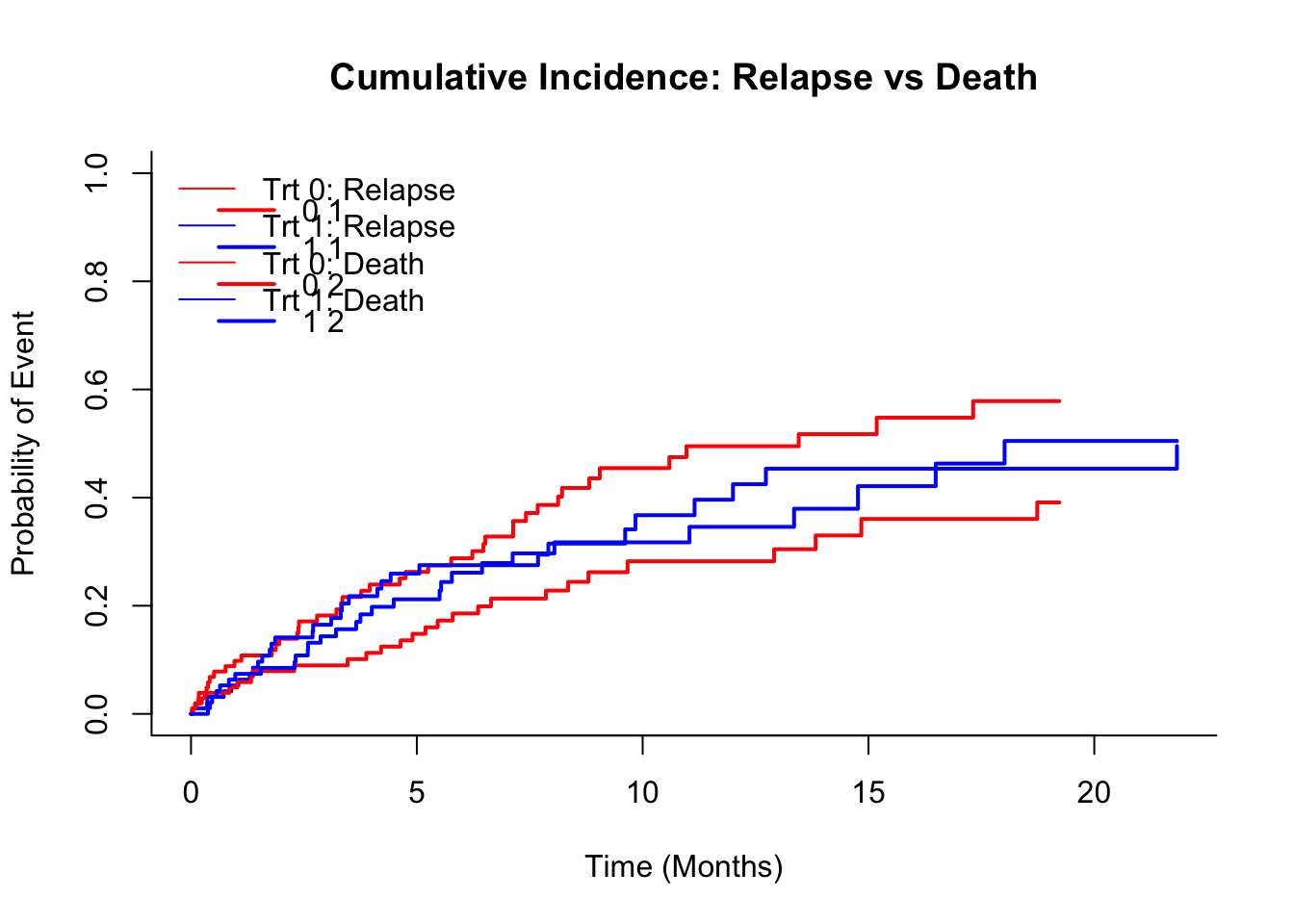
# --- 2. Estimate Cumulative Incidence Function (CIF) ---# We use the cuminc() function# ftime: failure time# ftype: failure status (1 is usually event of interest, 2 is competing risk)# group: grouping variable (optional, here we compare by Treatment)cif_fit <-cuminc(ftime = data$ftime, fstatus = data$ftype, group = data$trt)# Display the results at specific time pointsprint("Cumulative Incidence Estimates:")
# --- 3. Plotting the CIF ---# Plotting the Cumulative Incidence curvesplot(cif_fit, xlab ="Time (Months)", ylab ="Probability of Event", lwd =2, lty =1,col =c("red", "blue", "red", "blue"), # Colors for the curvesmain ="Cumulative Incidence: Relapse vs Death")legend("topleft", legend =c("Trt 0: Relapse", "Trt 1: Relapse", "Trt 0: Death", "Trt 1: Death"), col =c("red", "blue", "red", "blue"), lty =1, bty ="n")
# --- 4. Gray's Test ---# cuminc() automatically performs Gray's test for equality of CIFs across groups# The results are stored in the 'Tests' component of the fit objectprint("Gray's Test for Equality of CIFs:")
# --- 5. Fine-Gray Model (Subdistribution Hazards) ---# We use the crr() function (Competing Risks Regression)# It requires a design matrix for covariates (cov1)# Construct design matrix (excluding intercept)covariates <-model.matrix(~ trt, data = data)[, -1, drop =FALSE]# Fit model for Event of Interest (failcode = 1)# cencode = 0 indicates censored observationsfg_model <-crr(ftime = data$ftime, fstatus = data$ftype, cov1 = covariates, failcode =1, cencode =0)print("Fine-Gray Model Results (Event of Interest):")
[1] "Fine-Gray Model Results (Event of Interest):"
summary(fg_model)
Competing Risks Regression

Call:
crr(ftime = data$ftime, fstatus = data$ftype, cov1 = covariates,
    failcode = 1, cencode = 0)

      coef exp(coef) se(coef)     z p-value
trt -0.236      0.79    0.231 -1.02    0.31

    exp(coef) exp(-coef)  2.5% 97.5%
trt      0.79       1.27 0.502  1.24

Num. cases = 200
Pseudo Log-likelihood = -348
Pseudo likelihood ratio test = 1.02  on 1 df,
# Interpretation:# Exp(coef) is the Subdistribution Hazard Ratio (SHR).# If SHR < 1, the treatment reduces the cumulative incidence of relapse.
Interpretations in Statistics
Core Concepts & Statistical Interpretation
When analyzing time-to-event data where multiple mutually exclusive events can occur (e.g., Relapse vs. Death), standard survival analysis (Kaplan-Meier) is biased. We must distinguish between “rate” (speed) and “risk” (probability).
Cumulative Incidence Function (CIF)
Definition: The probability that a specific event \(k\) has occurred by time \(t\), accounting for the fact that other events may have prevented it.
Interpretation: “At 5 years, the cumulative incidence of relapse was 20%.” (Meaning 20% of the starting population had relapsed).
Contrast with KM: Kaplan-Meier estimates the risk in a hypothetical world where patients cannot die from other causes, which overestimates the risk of relapse in the real world.
Gray’s Test
Purpose: The “Log-Rank test” for competing risks.
Hypothesis: Tests if the Cumulative Incidence curves are identical between groups.
Interpretation: A p-value < 0.05 indicates a significant difference in the absolute risk of the event, but does not distinguish if this is due to treatment efficacy or toxicity (competing mortality).
The Two-Model Approach (Cox vs. Fine-Gray) To fully understand the drug’s effect, report both models:
Model
Metric
Interpretation
Use Case
Cause-Specific Cox
CS-HR
Biological Rate: “Among those alive and event-free, treatment changes the instantaneous rate of event by factor \(X\).”
Etiology / Mechanism
Fine-Gray
SHR
Prognostic Risk: “Treatment changes the cumulative probability of the event occurring by factor \(X\).”
Prediction / Resource Planning
The “Interpretation Trap”: False Benefit
A common paradox occurs when a treatment is highly toxic. It kills patients so quickly (Competing Risk) that they do not live long enough to experience the disease recurrence (Event of Interest).
The Scenario: “False Benefit”
Treatment: Highly Aggressive Chemotherapy.
Event 1 (Interest): Cancer Relapse.
Event 2 (Competing): Death from Toxicity/Infection.
The Paradoxical Results
Fine-Gray (SHR < 1): Suggests the treatment is Beneficial. (The probability of relapse is lower in the treatment group).
Cox (CS-HR\(\approx\) 1): Suggests the treatment is Useless. (It does not actually kill cancer cells any faster than control).
Cox for Death (CS-HR > 1): Suggests the treatment is Harmful. (It kills patients).
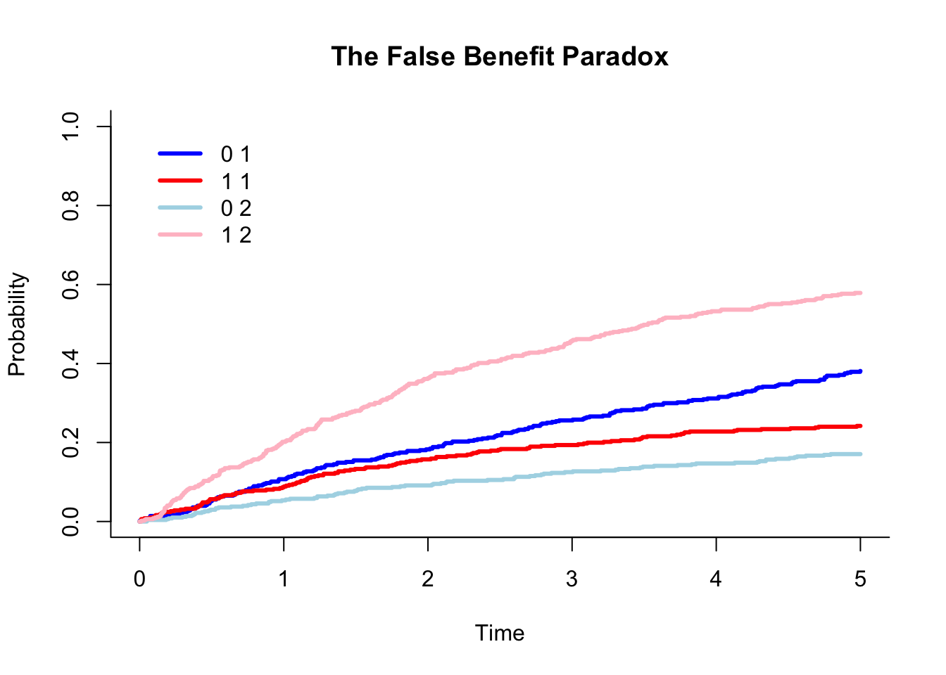
Conclusion: The lower relapse probability is an artifact of early death. This is a “False Benefit.”
R Code Demonstration: Simulating “False Benefit”
The following R code simulates a trial where the treatment has zero effect on cancer (Relapse hazard is identical) but high toxicity (Death hazard is 5x higher).
It demonstrates how the Cumulative Incidence curve for Relapse ironically looks better for the toxic treatment.
set.seed(999)n <-1000# Generate Treatment Group (0 = Control, 1 = Toxic Treatmenttrt <-rbinom(n, 1, 0.5)# --- 2. Define Hazards (The "Truth") ---# Both groups have SAME biological risk of Relapse (Event 1)lambda_relapse <-0.1# Treatment group has MUCH HIGHER risk of Death (Event 2 - Competing Risk)lambda_death_control <-0.05lambda_death_toxic <-0.25# 5x higher toxicity!# --- 3. Simulate Survival Times ---# We simulate latent times for both events and take the minimumftimes <-numeric(n)ftype <-numeric(n)for(i in1:n) {# Relapse time (Identical for both groups) t_relapse <-rexp(1, rate = lambda_relapse)# Death time (Depends on treatment toxicity) rate_death <-ifelse(trt[i] ==1, lambda_death_toxic, lambda_death_control) t_death <-rexp(1, rate = rate_death)# Determine which happens firstif(t_relapse < t_death) { ftimes[i] <- t_relapse ftype[i] <-1#Relapse } else { ftimes[i] <- t_death ftype[i] <-2# Death }}# Censor everyone at time 5 to emulate study endstudy_end <-5ftype[ftimes > study_end] <-0ftimes <-pmin(ftimes, study_end)# Create DataFramedata <-data.frame(id=1:n, time=ftimes, status=ftype, trt=trt)# --- 4. Statistical Analysis ---# A. Cause-Specific Cox Model (Biological Effect)# We censor deaths (status=2) when analyzing relapse (status=1)cox_relapse <-coxph(Surv(time, status==1) ~ trt, data=data)# B. Fine-Gray Model (Prognostic Risk)fg_relapse <-crr(data$time, data$status, data$trt, failcode=1,cencode=0)# --- 5. Output Results ---cat("\n=== TRUE BIOLOGICAL EFFECT (Cox Model)===\n")
=== TRUE BIOLOGICAL EFFECT (Cox Model)===
cat("Expected HR approx 1.0 (No benefit)\n")
Expected HR approx 1.0 (No benefit)
print(summary(cox_relapse)$coefficients)
           coef exp(coef)  se(coef)          z  Pr(>|z|)
trt -0.07945519 0.9236194 0.1174056 -0.6767581 0.4985595
In clinical trials where death or other terminating events are common (e.g., oncology, cardiology, geriatrics), ignoring competing risks can lead to inflated efficacy estimates.
* Use Cause-Specific Hazards to understand biological drivers.
* Use Cumulative Incidence (CIF) / Fine-Gray to predict actual patient outcomes and risks.